Produce awesome plots using ggplot2 - rochevin/formation_ggplot2_2023 GitHub Wiki
p_raster <- iris.tbl %>% ggplot(aes(y=Part,x=Individual,fill=obs)) + geom_raster() + facet_wrap(~Metric) + scale_fill_viridis_c()
p_raster
pos_end_species <- iris.tbl %>% group_by(Species) %>% arrange(Individual) %>% slice(1)
p_raster + scale_x_continuous(breaks = pos_end_species$Individual,labels = pos_end_species$Species)
p_raster_2 <- iris.tbl %>%
  unite(Feature,Part,Metric)%>%  #Remerge into one column
  group_by(Species) %>% mutate(Ind_spe = 1:dplyr::n()) %>%  # Create Ind label but by species
  ggplot(aes(y=Species,x=Ind_spe,fill=obs)) + geom_raster() + facet_wrap(~Feature,scales="free_x") + scale_fill_viridis_c()
p_raster_2
iris.tbl %>% ggplot(aes(x=obs,y=..density..,col=Species)) + geom_histogram(bins=50) + geom_density() + facet_wrap(Part~Metric)
By calling within a geom_*:
p1_bar <- iris.tbl %>% unite(Feature,Part,Metric) %>% ggplot(aes(x=Species,y=obs,fill=Feature)) +
  geom_bar(col="black",position="dodge",stat = "summary", fun = "mean")+ scale_fill_viridis_d(option="plasma") +
  coord_cartesian(expand = F)
p1_bar
Or by using it directly:
p2_bar <- iris.tbl %>% unite(Feature,Part,Metric) %>% ggplot(aes(x=Species,y=obs,fill=Feature)) +
  stat_summary(geom = "bar",position = "dodge",fun.y = "mean",col="black") + scale_fill_viridis_d(option="plasma") +
  coord_cartesian(expand = F)
## Warning: `fun.y` is deprecated. Use `fun` instead.
p2_bar
You can also do it before plotting using stat="identity"
p3_bar <- iris.tbl %>% unite(Feature,Part,Metric) %>% group_by(Species,Feature) %>% summarise(mean=mean(obs)) %>%
  ggplot(aes(x=Species,y=mean,fill=Feature)) + geom_bar(col="black",stat="identity",position="dodge") + scale_fill_viridis_d(option="plasma")
## `summarise()` has grouped output by 'Species'. You can override using the
## `.groups` argument.
p3_bar
You can also add standard deviation:
p4_bar <- iris.tbl %>% unite(Feature,Part,Metric) %>% ggplot(aes(x=Species,y=obs,fill=Feature)) +
  stat_summary(geom = "bar",position = "dodge",fun = "mean",col="black") + scale_fill_viridis_d(option="plasma") +
  stat_summary(fun.data=mean_sdl,geom = "errorbar",position="dodge") +
  coord_cartesian(expand = F)
p4_bar
iris %>% ggplot(aes(x=Petal.Length,y=Petal.Width)) + geom_point()
iris %>% ggplot(aes(x=Petal.Length,y=Petal.Width)) + geom_point(aes(col=Species))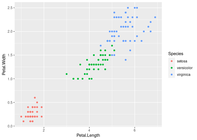
iris %>% ggplot(aes(x=Petal.Length,y=Petal.Width))  +
  geom_point(stat = "summary",fun = "mean",col="black",size = 4) +
  stat_summary(fun.data=mean_sdl,geom = "errorbar") +
  geom_point(aes(col=Species))
iris %>% ggplot(aes(x=Petal.Length,y=Petal.Width))  +
  geom_point(stat = "summary",fun = "mean",col="black",size = 4) +
  stat_summary(fun.data=mean_sdl,geom = "errorbar") +
  geom_line(stat = "summary",fun = "mean",col="black") +
  geom_point(aes(col=Species))
If you have continous value, you can plot a line with geom_line and
plotting the standard deviation using geom_ribbon
iris %>% ggplot(aes(x=Petal.Length,y=Petal.Width))  +
  stat_summary(fun.data=mean_sdl,geom = "ribbon",alpha=0.4) +
  geom_line(stat = "summary",fun = "mean",col="black") +
  geom_point(aes(col=Species))
iris %>% ggplot(aes(x=Petal.Length,y=Petal.Width))  +
  geom_point()+
  geom_smooth(method = "lm")
## `geom_smooth()` using formula 'y ~ x'

iris %>% ggplot(aes(x=Petal.Length,y=Petal.Width))  +
  geom_point()+
  geom_smooth(method = "loess")
## `geom_smooth()` using formula 'y ~ x'

iris %>% ggplot(aes(x=Petal.Length,y=Petal.Width))  +
  geom_point()+
  geom_smooth(method = "lm",formula = y ~ log(x))
iris %>% ggplot(aes(x=Petal.Length,y=Petal.Width,col=Species))  +
  geom_point()+
  geom_smooth(method = "lm")
## `geom_smooth()` using formula 'y ~ x'

iris %>% ggplot(aes(x=Petal.Length,y=Petal.Width))  +
  geom_point(aes(col=Species))+
  geom_smooth(method = "lm")
## `geom_smooth()` using formula 'y ~ x'

pca.iris <- prcomp(dplyr::select(iris,-Species),scale=TRUE,center=TRUE)percent_var_explained <- tibble(
PC=1:ncol(pca.iris$x),
percent_Var=(pca.iris$sdev^2 / sum(pca.iris$sdev^2)),
cumsum_Var = cumsum(percent_Var)
)
pca.p1 <- percent_var_explained %>%
ggplot(aes(x=PC,y=percent_Var)) +
geom_bar(stat="identity") +
geom_line(aes(y=cumsum_Var),group=1) +
geom_point(aes(y=cumsum_Var),col="red") +
ggrepel::geom_label_repel(aes(y=cumsum_Var,label = scales::percent(cumsum_Var)),direction="y") +
labs(
x = "**Principal Component** <br>(PC)",
y = "**Contribution** <br>(Variance explained in %)"
) +
scale_y_continuous(labels = scales::percent) +
theme(
axis.title.x = ggtext::element_markdown(),
axis.title.y = ggtext::element_markdown()
)
pca.p1
pca.iris.tibble <- bind_cols(
  iris %>%  dplyr::select(Species),
  pca.iris$x %>% setNames(glue::glue("PC{1:4}"))
)

pca.p2 <- pca.iris.tibble %>% ggplot(aes(x=PC1,y=PC2,fill=Species,label=Species)) +
  geom_point() + ggforce::geom_mark_hull()
pca.p2
require(patchwork)## Le chargement a nécessité le package : patchwork
pca.p1 + pca.p2 + plot_layout(width=c(0.4,0.6))
iris.tbl  %>%
  ggplot(aes(x = Species, y = obs,col=Species,fill = after_scale(colorspace::lighten(color, .5)))) +
  ggdist::stat_halfeye(
    adjust = .5,
    width = .6,
    .width = 0,
    justification = -.2,
    point_colour = NA
  ) +
  geom_boxplot(
    width = .15,
    outlier.shape = NA
  ) +
  ## add justified jitter from the {gghalves} package
  gghalves::geom_half_point(
    ## draw jitter on the left
    side = "l",
    ## control range of jitter
    range_scale = .4,
    ## add some transparency
    alpha = .3
  ) + facet_grid(Part~Metric)
iris_ratio <- iris %>%
  mutate(Ind = 1:dplyr::n()) %>%
  gather(key="Feature",value ="value",-Species,-Ind) %>%
  separate(Feature,into = c("Feature","Measure"),sep = "\\.") %>%
  spread(key = Measure,value=value) %>% mutate(ratio = log2(Length/Width)) %>%
  group_by(Species,Feature) %>%
  mutate(
    n = dplyr::n(),
    median = median(ratio),
    max = max(ratio)
  ) %>%
  ungroup() %>%
  mutate(species_num = as.numeric(Species))


p_stat <- iris_ratio %>%
  ggplot(aes(y=Species,x=ratio,color=Species)) +
  stat_summary(
    geom = "linerange",
    fun.min = function(x) -Inf,
    fun.max = function(x) median(x, na.rm = TRUE),
    linetype = "dotted",
    orientation = "y",
    size = .7
  ) +
  geom_point(
    aes(y = species_num - .12),
    shape = "|",
    size = 2,
    alpha = .33
  )  +
  ggridges::geom_density_ridges(aes(fill = Species),scale=0.9,alpha=0.7) +
  ggdist::stat_pointinterval(
    aes(
      y = species_num,
      color = Species,
      fill = after_scale(colorspace::lighten(color, .5))
    ),
    shape = 18,
    point_size = 3,
    interval_size = 1.8,
    adjust = .5,
    .width = c(0, 1)
  ) +
  geom_text(
    aes(x = median, label = format(round(median, 2), nsmall = 2)),
    stat = "unique",
    color = "white",
    family = "Open Sans",
    fontface = "bold",
    size = 3.4,
    nudge_y = .15
  ) +
  geom_label(
    aes(x = max, label = glue::glue("n = {n}")),
    stat = "unique",
    family = "Open Sans",
    fontface = "bold",
    size = 3.5,
    hjust = 0,
    nudge_x = .05,
    nudge_y = .02
  ) +
  facet_wrap(~Feature) +
  coord_cartesian(clip="off")

p_stat
## Picking joint bandwidth of 0.116
## Picking joint bandwidth of 0.0502

dataset <- "DE_result_edgeR_1_0.05_CvsC_OHT_table.tsv"
dataset <- dataset %>% read_tsv()
## Rows: 12382 Columns: 9
## ── Column specification ────────────────────────────────────────────────────────
## Delimiter: "\t"
## chr (2): rowname, Gene.name
## dbl (7): logFC, logCPM, LR, PValue, p.adj, FILTER.FC, FILTER.P
##
## ℹ Use `spec()` to retrieve the full column specification for this data.
## ℹ Specify the column types or set `show_col_types = FALSE` to quiet this message.
## # A tibble: 12,382 × 9
## rowname logFC logCPM LR PValue p.adj FILTER.FC FILTER.P Gene.name
## <chr> <dbl> <dbl> <dbl> <dbl> <dbl> <dbl> <dbl> <chr>
## 1 ENSG000000… -0.00411 4.65 0.00101 0.975 1.00 0 0 TSPAN6
## 2 ENSG000000… 0.0447 5.30 0.159 0.690 1.00 0 0 DPM1
## 3 ENSG000000… -0.0252 2.78 0.0215 0.883 1.00 0 0 SCYL3
## 4 ENSG000000… -0.0467 4.78 0.0998 0.752 1.00 0 0 C1orf112
## 5 ENSG000000… 0.351 1.22 1.04 0.308 0.939 0 0 CFH
## 6 ENSG000000… -0.0307 5.56 0.0581 0.810 1.00 0 0 FUCA2
## 7 ENSG000000… -0.0262 5.27 0.0509 0.822 1.00 0 0 GCLC
## 8 ENSG000000… 0.0491 5.67 0.188 0.665 1.00 0 0 NFYA
## 9 ENSG000000… -0.254 2.78 2.23 0.135 0.736 0 0 STPG1
## 10 ENSG000000… -0.178 5.05 1.89 0.169 0.794 0 0 NIPAL3
## # … with 12,372 more rows
-
rowname: gene ID (Ensembl). -
logFC: log2 ratio between expression of the treatment and the control condition. -
logCPM: average expression for this gene. -
p.adj: is the logFC significant ? -
Gene.name: Name of the gene.
dataset %>% ggplot(aes(x=logFC,y=-log10(p.adj))) +
  geom_point() +
  coord_cartesian(xlim=c(-2,2)) +
  geom_hline(yintercept = -log10(0.05),linetype="dashed") +
  geom_vline(xintercept = c(-1,1),linetype="dashed")
dataset <- dataset %>% mutate(Type = case_when(
  p.adj< 0.05 & logFC > 1 ~ "Upregulated",
  p.adj< 0.05 & logFC < -1 ~ "Downregulated",
  TRUE ~ "None"
))
dataset %>% count(Type)
## # A tibble: 3 × 2
## Type n
## <chr> <int>
## 1 Downregulated 12
## 2 None 12314
## 3 Upregulated 56
dataset %>% ggplot(aes(x=logFC,y=-log10(p.adj))) +
  geom_point(aes(col=Type)) +
  coord_cartesian(xlim=c(-2,2)) +
  geom_hline(yintercept = -log10(0.05),linetype="dashed") +
  geom_vline(xintercept = c(-1,1),linetype="dashed")
require(glue)## Le chargement a nécessité le package : glue
dataset <- dataset %>% group_by(Type) %>% mutate(number_Type = dplyr::n()) %>%
mutate(Type_nb = glue("{Type} ({number_Type})"))require(ggtext)## Le chargement a nécessité le package : ggtext
dataset <- dataset %>% mutate(color = case_when(
  Type == "Upregulated" ~ "#c0392b",
  Type == "Downregulated" ~ "#2980b9",
  TRUE ~ "#535c68"
)) %>%
  mutate(Type_nb = as.factor(glue("<i style='color:{color}'>{Type}</i> ({number_Type})")))
p1 <- dataset %>% ggplot(aes(x=logFC,y=-log10(p.adj))) +
geom_point(aes(col=color)) +
scale_color_identity(labels=levels(dataset$Type_nb),guide="legend") +
geom_hline(yintercept = -log10(0.05),linetype="dashed") +
geom_vline(xintercept = c(-1,1),linetype="dashed") +
theme(legend.text = element_markdown())
p1
Here we need the top 15 of each category
require(ggrepel)## Le chargement a nécessité le package : ggrepel
dataset_label <- dataset %>% filter(Type != "None") %>%
  group_by(Type) %>% arrange(desc(abs(logFC))) %>%  slice(1:15)


p2 <- p1 + geom_label_repel(data=dataset_label,aes(label=Gene.name,col=color),fill=NA,box.padding = 1,max.overlaps = Inf,show.legend = F)theme_set(theme_classic(base_size=12,base_family = "Open Sans"))
theme_update(legend.text = element_markdown(),
legend.position ="bottom",
plot.title.position = "plot",
plot.caption.position = "plot",
plot.title = ggtext::element_markdown(),
plot.subtitle = ggtext::element_markdown(),
plot.caption = ggtext::element_markdown(),
legend.title = ggtext::element_markdown(),
axis.title.x = ggtext::element_markdown(),
axis.title.y = ggtext::element_markdown()
)
p2 + labs(
title = "Differential expression analysis after **DNA double-strand break damage induction**",
subtitle = 'from RNA-seq data between two conditions : *OHT* (DSB damage induction) and *untreated*.',
caption = "Data accession **E-MTAB-6318**",
x = "**Fold-Change** after damage induction <br>(Log2)",
y = "**Adjusted P-value** <br>(-log10)",
color = "Fold-change <br>(categorical)"
)## Warning: Removed 1 rows containing missing values (geom_label_repel).
