Time response - quangounet/open-control-theory GitHub Wiki
Before starting, make sure to load the required packages.
Type (or copy-paste) the following code into the ipython
command prompt
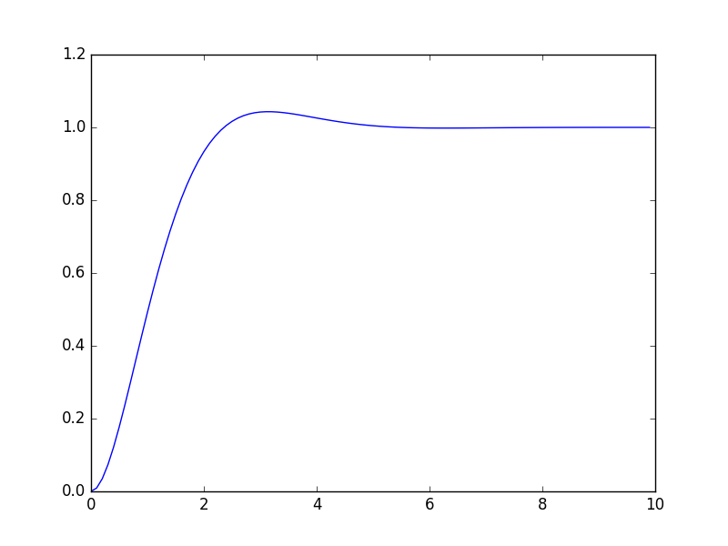
sys = tf([2], [1, 2, 2]) # Define a transfer function C/R = 2/(s^2+2s+2)
Tv = arange(0, 10, 0.1) # Define simulation window between t=0 and t=10 with 0.1 increment
Cstep, _ = step(sys, T=Tv) # Compute step response
plot(Tv, Cstep) # Sketch the step response
The following figure should pop up

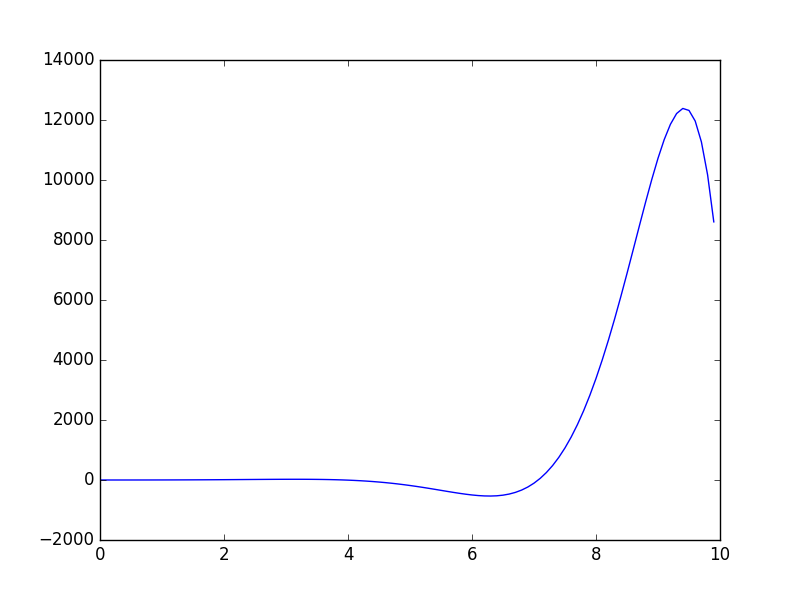
sys2 = tf([2], [1, -2, 2]) # Define a transfer function C/R = 2/(s^2-2s+2)
Tv = arange(0, 10, 0.1) # Define simulation window between t=0 and t=10 with 0.1 increment
Cstep2, _ = step(sys2, T=Tv) # Compute step response
clf() # Clear the figure before plotting a new one
plot(Tv, Cstep2) # Sketch the step response
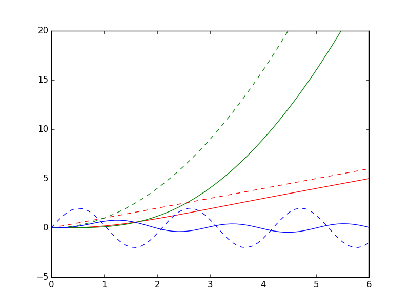
For other types of input (ramp, parabola, sine waves, etc.), one needs to define explicitly the input vectors.
sys = tf([2], [1, 2, 2]) # Define a transfer function C/R = 2/(s^2+2s+2)
Tv = arange(0, 10, 0.1) # Define simulation window between t=0 and t=10 with 0.1 increment
Rramp = Tv # Unit ramp input
Rparabola = [t*t for t in Tv] # Unit parabola input
Rsine = [2*sin(3*t) for t in Tv] # Sine input
_, Cramp, _ = forced_response(sys, T=Tv, U=Rramp) # Compute ramp response
_, Cparabola, _ = forced_response(sys, T=Tv, U=Rparabola) # Compute parabola response
_, Csine, _ = forced_response(sys, T=Tv, U=Rsine) # Compute sine response
clf() # Clear the figure before plotting a new one
plot(Tv, Rramp, "r--", Tv, Cramp, "r" ) # Plot ramp input and response in red
plot(Tv, Rparabola, "g--", Tv, Cparabola, "g") # Plot parabola input and response in green
plot(Tv, Rsine, "b--", Tv, Csine, "b") # Plot sine input and response in blue
axis([0, 6, -5, 20]) # Restricts the plot to t = [0, 6]