I. Introduction
II. Importing Agisoft wavefront object
III. Decimating the mesh
IV. Sculpting the mesh
V. Refining the texture
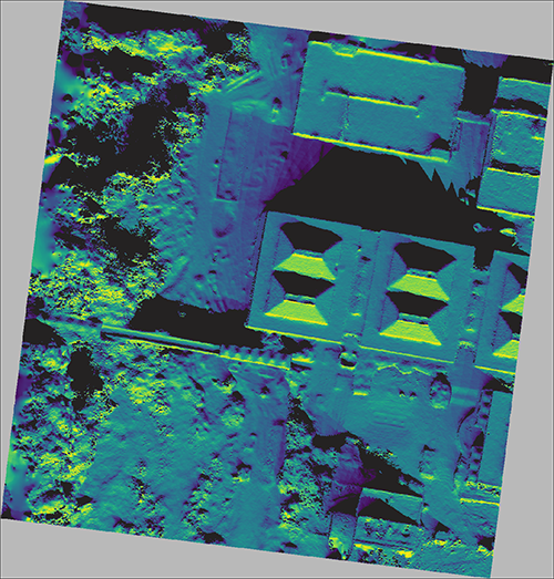
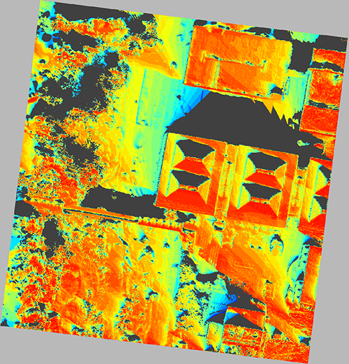
VI. Draping GIS analysis maps
VII. Importing Digital Surface model (DSM)

• Download and install latest version of Blender from here.
• Download and install Blender GIS addon from here. Installation guide available here.
• Download and unpack sample_data folder from here

---

orthophoto	relief	aspect
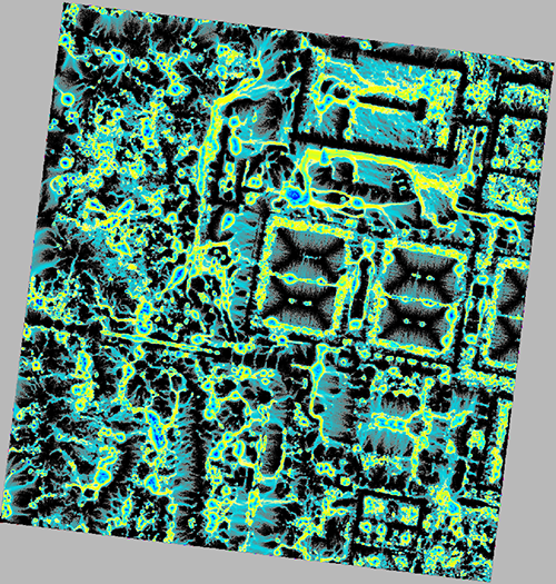Waterflow	Solar analysis (irradiance map)	Solar analysis (insolation time)

In this tutorial, we will get familiar with techniques for importing, processing and rendering UAS data. The sample data at hand consists of a 3D mesh, a digital surface model (DSM) and series of analysis maps. Mesh and Digital surface models has been generated in AGISoft from UAV nadir and NSWE oblique imagery (250ft) and analysis has been performed in GRASS GIS. Get the full report of the flight survey here.

---

• Run Blender and open the file centennial_uav.blend.
• Make sure that Render engine is set to Cycles Render. You can find the option in the viewport's top header.

---

Wavefront object (.obj) is perhaps the most common 3D mesh format, and a very efficient way to transfer the object's geometry and the material. When exporting UAS meshes to wavefront, the mesh geometry is saved in a .Obj file, the texture information in an image file (e.g., Jpeg, PNG), and the material information in a (.mtl) file. The only drawback of Obj files is loss of georeferencing, meaning that when imported in other software they will be located in an arbitrary or software selected origin. In this step, we will import the mesh file.

• Go to File > Import > Wavefront objects (.obj) and browse to the sample_data folder
• Select the centennial_OBJ.obj
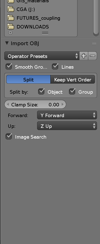
• In the import options (bottom left side of the import):
  • Change the direction to Z up and Y forward (see figure below, left). These parameters are adjusted to the axis direction of the 3D space. For example, Z up means that the height axes is defined as Z with positive up.
  • Make sure that the Image search option is activated so you import the mesh and the material.
  • Press enter to finalize the import. Your imported object should look like the image below on the right.
• Switch between Wire, Solid and Material shading modes to examine the surface quality.

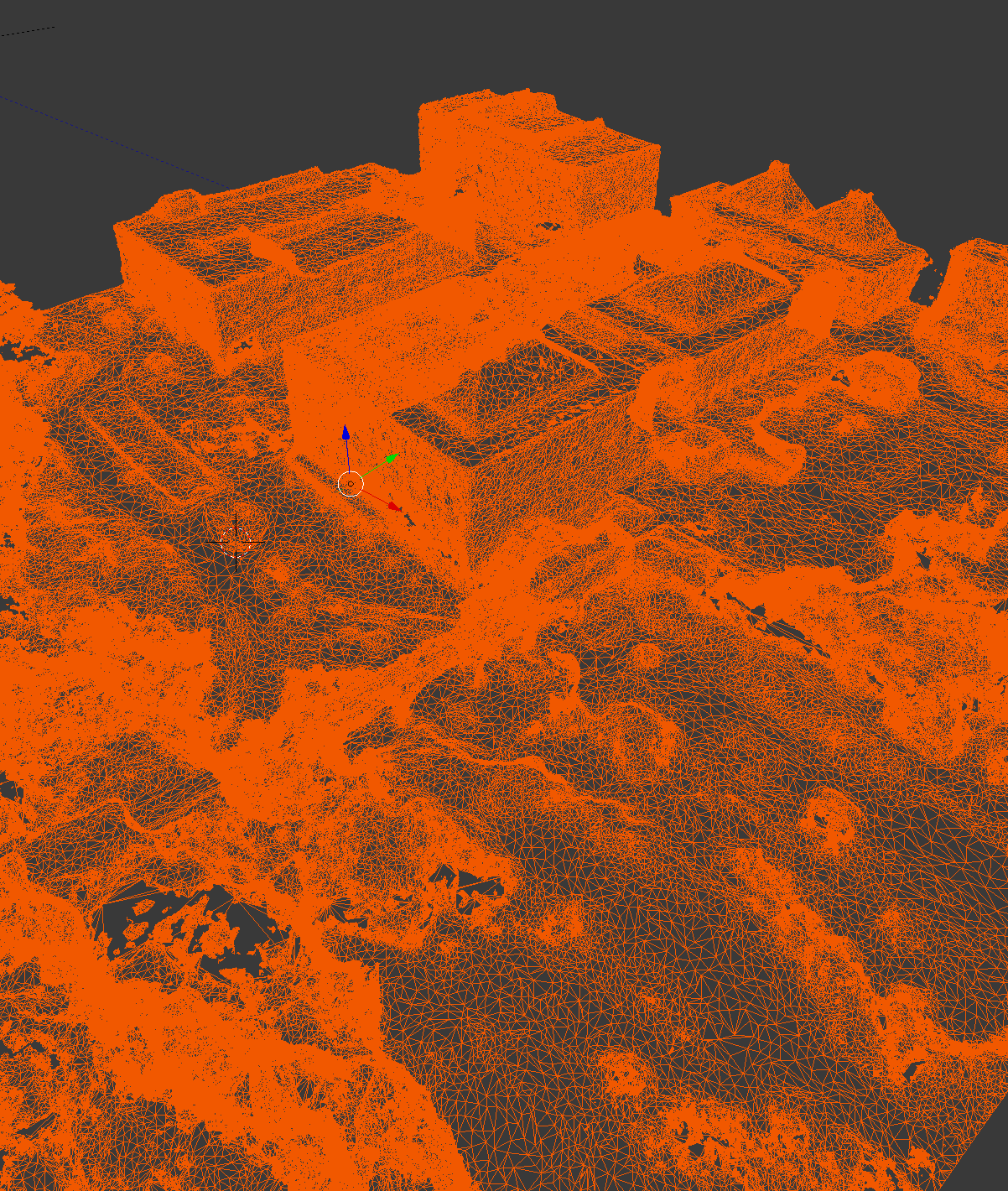Wavefront Imported mesh object	imported object

---

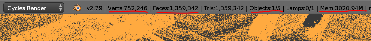Viewport top header showing the scene complexity and memory consumption information

3D meshes exported from Agisoft or similar photogrammetry software are usually very dense and contain millions of faces draining exorbitant amount of memory, storage and processing resources. It is possible to decimate them without loosing the surface details. In this step we will use Decimate modifier to decimate the imported mesh.

In Blender, you can track real-time information about the total number of faces in the scene as well as their consumed memory from 3D viewport's top header (see figure above).

• Select the imported object (centennial_OBJ).
• Change the viewport shading mode to Wire so you have a better view of the mesh structure.
• Go to Properties Editor > Modifiers tab > Add Modifier > from the dropdown select Decimate(figure below, left). You will see the decimate panel show up in the properties editor. Notice that the current face count of the object is indicated as 1371299 (figure below, right).
• Click on the Ratio slider and type in 0.5 (figure below, right). Wait for the process to finish, it may take several seconds depending on your system's computation power.
  Note: Do not drag the Ratio slider to avoid freezing and crashes. Use keyboard input instead.
• You will notice that the face count is reduced to half (685645) and the wireframe shows that the polygons are spaced out.
• Switch the viewport shading to Material to examine the quality loss.
• In Decimate modifier's panel click on Apply to finalize the modification. This process may also take several seconds.

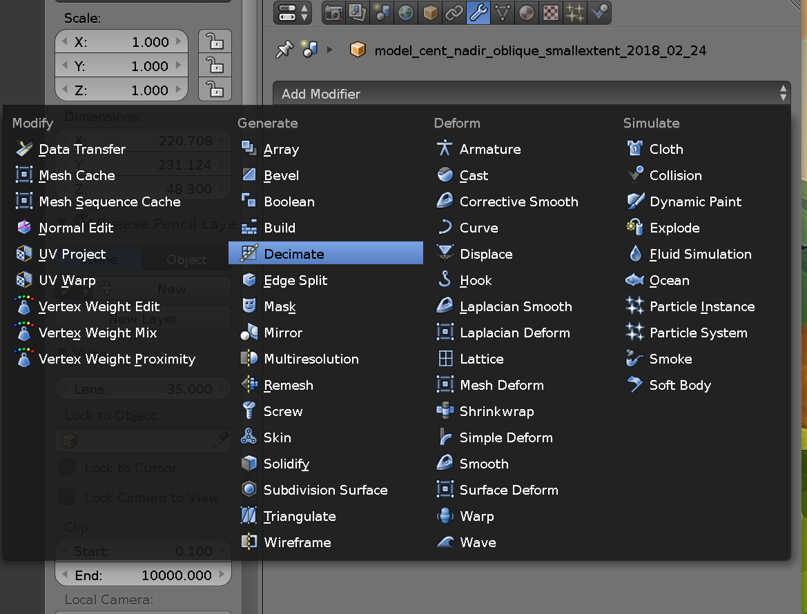Decimate modifier accessed from the Properties Editor, Modifiers tab	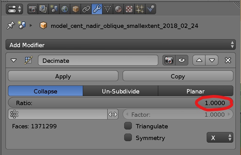Decimate modifier panel

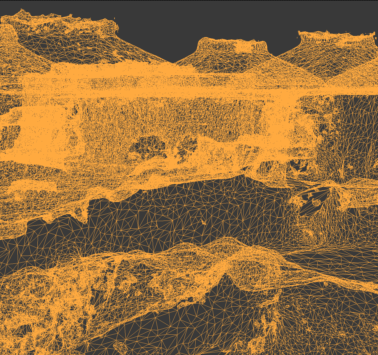Before decimation	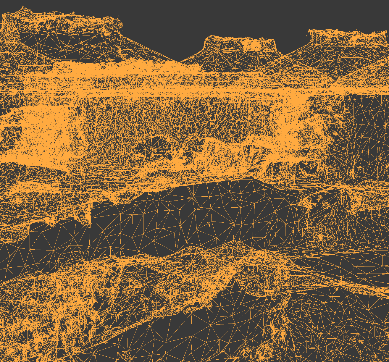After decimation to 0.5 face count

---

Blender comes with comprehensive sculpting tools that can be used to make local mesh refinements such as leveling a surface, filling a whole, removing the dents, etc.
Note: Sculpting tools are useful for treating existing faces, thus they cannot be used to fill large wholes or reconstruct big chunks of missing data.

• Select the centennial_OBJ object.
• Change the viewport shading mode to Solid so you can better see the surface quality.
• From the viewport's bottom header > switch from Object Mode to Sculpt Mode. The sculpting panel will show up in viewport's left toolbar in the Tools tab (figure below).
• Pick an area of your choosing that needs treatment to start experimenting with different brushes.
• General procedure for using sculpting brushes is as following:
  • In the sculpting toolbar, click on the Brush thumbnail to see the list of Brushes > select a brush.
  • Each brush has a different functionality some examples follow:
    • Inflate/Deflate can be used for extruding depressions or decompressing bumps. You can switch between Inflate and Deflate in the toolbox.
    • Smooth can be used for leveling and smoothing surfaces.
    • Snake Hook can be used for dragging the vertices to and close the gaps.
  • Once the brush is selected, hover the mouse over the treatment area in 3D view and click to apply the brush. You can click and drag to continuously apply the treatment.
  • To change the brush stroke parameters:
    • Adjust the Radius parameter to increase/decrease the brush size (keyboard shortcut [ and ]).
    • Adjust the Strength parameter to increase/decrease the magnitude of the effect.
  • To snap the brush stroke to a specific direction:
    • Collapse Symmetry/Lock section and select X, Y or Z parameters.
  • Switch back the object interaction mode to Object Mode.

Sculpt mode selected from bottom header and Sculpting tools appeared in the left toolbar

Sculpting brushes

Mesh surface before sculpting	Mesh surface after sculpting

The UAV derived textures often include small imperfections such as black voids. These errors can be partially corrected using Texture paint tool. Consider Texture Paint as a small photo editing software that allows for editing the textures draped onto the 3D mesh. Like sculpting tools texture paint has variety of brush types. In this tutorial we will only use Clone brush. As the name suggest, Clone tool copies color information from one area as reference and applies it to another area. The procedure is as follows:

• Select the centennial_OBJ object. viewport's left toolbar in the Tools tab (figure below).
• Zoom-in on an area of your choosing that needs treatment.
• From the viewport's bottom header > switch from Object Mode to Texture Paint. The texture paint panel will show up in up in viewport's left toolbar in the Tools tab.
• In the texture paint toolbar, click on the Brush thumbnail to see the list of Brushes > select Clone.
• Increase/decrease the size of the Brush using the Radius parameter (keyboard shortcut [ and ])
• To apply the clone brush:
  • Hold Ctrl key and click on the area that the reference color needs to be picked.
  • Hover the mouse to the area that needs treatment and left-click to paint.

Note: Texture paint can be only applied to areas that have geometry but miss color information. Don't expect to fill-in the mesh voids with this tool.

Sculpting brushes

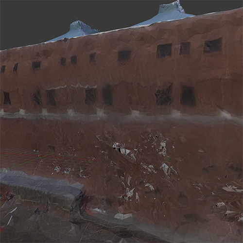Before applying texture paint	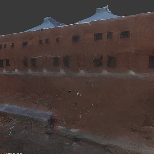After applying texture paint

In this step, we drape various analysis maps including Solar analysis, Water flow simulation, aspect and relief on the mesh surface using Node editor. The workflow for creating each material includes removing the existing material, creating a new one and setting up the node network, as discussed in the advanced shading topic. Below we exemplify the step-by-step procedure for draping one of the textures (Solar analysis) and for the rest we provide the Node network so you can reconstruct them yourself.

• Some general tips before starting:
  • Make sure that your render engine is set to Cycles render.
  • Save your blender file throughout the process.
  • If you don't have a fast processing computer, do not attempt to change node options, while in viewport rendering mode. Finalize your modifications in Material mode and then switch to render.

For draping the solar analysis we simply create an Image Texture node assigned through Diffuse BSDF node to the object surface.

• To remove the existing material and create a new one:

  • Select the centennial_OBJ object.
  • Go to Properties editor > Material > select the material in the material slot > Press - button to remove the material from the slot.
  • If there is more than one material in the slot, remove all of them to clear the slot.
  • Create a new material using the + button and rename it (e.g., water flow)

• To add the Solar analysis as a Texture Image:

  • In the Node editor, bottom header click on Add menu and go to Texture > Image Texture.
  • In the Texture node Click on the folder icon to browse a new image.
  • Navigate to the folder sample_data > Select irradiance.jpg.
  • From the Node editor, bottom header click on Add menu and go to Input > Texture Coordinate.
  • Connect the Generated output to the Vector input of the Image Texture node.
  • Connect the Color output of the Image Texture node to Color output of the Diffuse node.

  
  
  Node network of the solar analysis material

  
  

  
  
  Rendering

  
  

We can overlay Waterflow map one the orthophoto to show the context or on an aspect map to accentuate the surface roughness using a Mix shader node. The null areas in the waterflow map is black allowing us to make them transparent using a Transparent node. When transparent node is linked to the mix shader's factor input, the black areas of the first node (waterflow) will be masked and replaced with the second node (aspect). The node structure is shown below. You can replace the ortho image with aspect.

Node network of the waterflow material. Added nodes are highlighted in red.

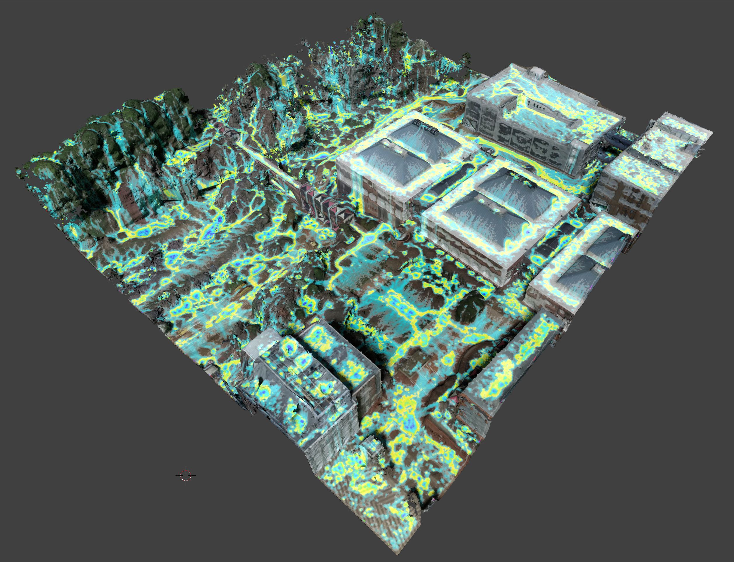Rendering of the water flow mixed with ortho image	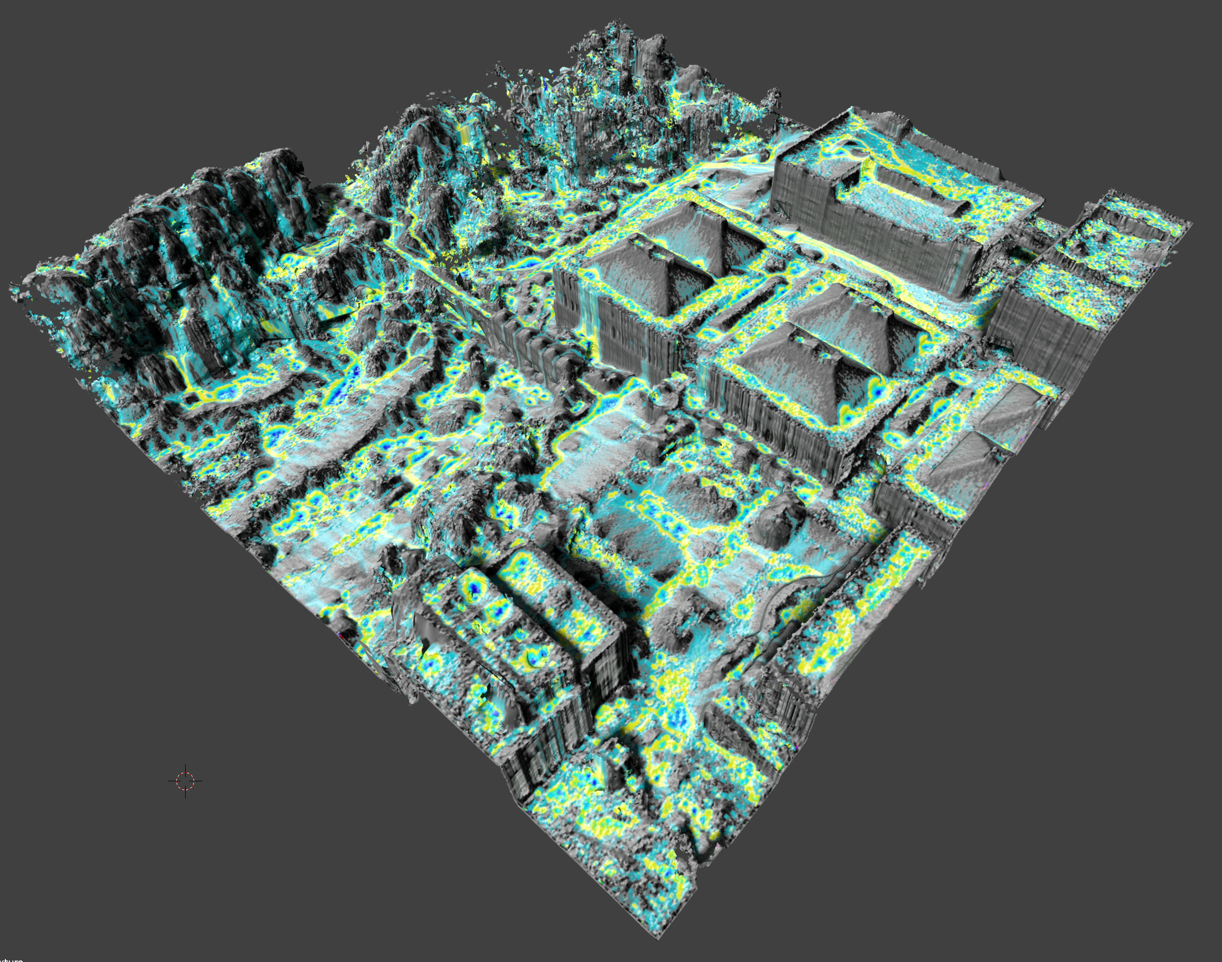Rendering of the water flow mixed with aspect map

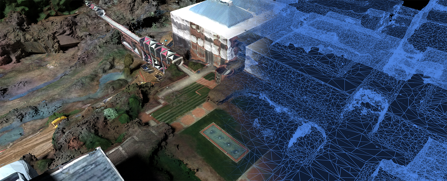
A holographic rendering is an engaging technique for representing mesh structure. Because holograms are essentially photographic recording of a light field, they can be mimicked through glowing and faded wireframe type renderings. Here, we represent these effects through a combination of emission, Transparent and Wireframe Nodes. Additionally, we blend it with an orthophoto and connect the transition line to the camera, so that we continuously interface between the skinned and naked mesh representation as we orbit around the mesh in the 3D viewport. Once you reconstructed the node network, play with the highlighted parameters to explore how they influence the representation.

Node network of the transitioning hologram material. The background frames are only for clarity purposes and don't have any effect on the object material.

Rendering of the blended hologram material

In this step, we will learn how to setup blender GIS addon and georeference the scene. Then, we will go over the workflow for importing and processing DSMs. Finally, we will juxtapose the DSM and wavefront meshes to compare their surface representation quality.

• Download the BlenderGIS addon
• Go to file ‣ user preferences ( Alt + Ctrl + U ) ‣ Add-ons ‣ Install from File (bottom of the window)
• Browse and select "BlenderGIS-master.zip" file
• You should be able to see the addon 3Dview: BlenderGIS added to the list. If not, type "gis" in the search bar while making sure that in the Categories panel All is selected. In the search results you should be able to see 3Dview: BlenderGIS. Select to load the addon.
• From the bottom of the preferences window click Save User Settings so the addon is saved and automatically loaded each time you open blender

Before setting up the coordinate reference system of the Blender scene and configuring the scene projection, you should know the Coordinate Reference System (CRS) and the Spatial Reference Identifier (SRID) of your project. You can get the SRID from http://epsg.io/ or spatial reference website using your CRS. The example datasets in this exercise uses a NAD83(HARN)/North Carolina CRS (SSRID EPSG: 3358). Learn more about Georeferencing management in Blender Here .

• In BlenderGIS add-on panel (in preferences windows), select to expand the 3D View: BlenderGIS
• In the preferences panel find Spatial Reference Systems and click on the + Add button
• In the add window type in 3358 for definition and "NAD83(HARN)/North Carolina" for Description. Then select Save to addon preferences
• Select OK and close the User Preferences window.

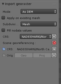Georaster import parameters

Installing addon and setting up Coordinate System

Rasters can be imported and used in different ways. You can import them As DEM to use it as a 3D surface or as Raw DEM to be triangulated or skinned inside Blender. You can select On Mesh to drape them as a texture on your 3D meshes. In this example, we import a digital surface model (DSM) derived from Lidar data points dataset as a 3D mesh using As DEM method. Note: Blender GIS imports both Digital Elevation Model (DEM) and Digital Surface Model (DSM) through As DEM method.

• Hide the existing (centennial_OBJ) object in the outliner (click on the eye and camera icons).
• Go to file ‣ import ‣ Georeferenced Raster
• On the bottom left side of the window find Mode and select As DEM
• Set subdivision to Subsurf and select NAD83(HARN) for georeferencing
• Browse to the 'sample_data' folder and select centennial_dsm.tif
• Click on Import georaster on the top right header
• If all the steps are followed correctly, you should be able to see the terrain in 3D view window

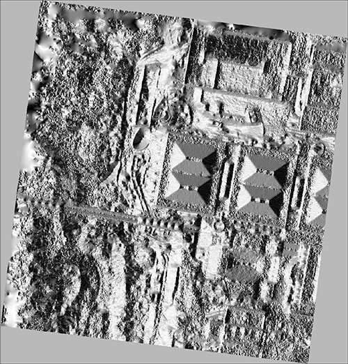
Usually when surface or elevation models are imported in Blender they are downsampled to a default subdivision resulting in a smoothed generalized surface. The following procedure subdivides the polygons of the imported surface to acquire a more detailed mesh.

• Select the centennial_dsm object
• Go to 3D view editor's bottom toolbar ‣ Object interaction mode ‣ Edit Mode
• Switch to Face select
• If object is not orange in color (i.e., nothing is selected), go to Select ‣ (De)select All (or press A) to select all faces (when the object faces are selected, they will be highlighted in orange).
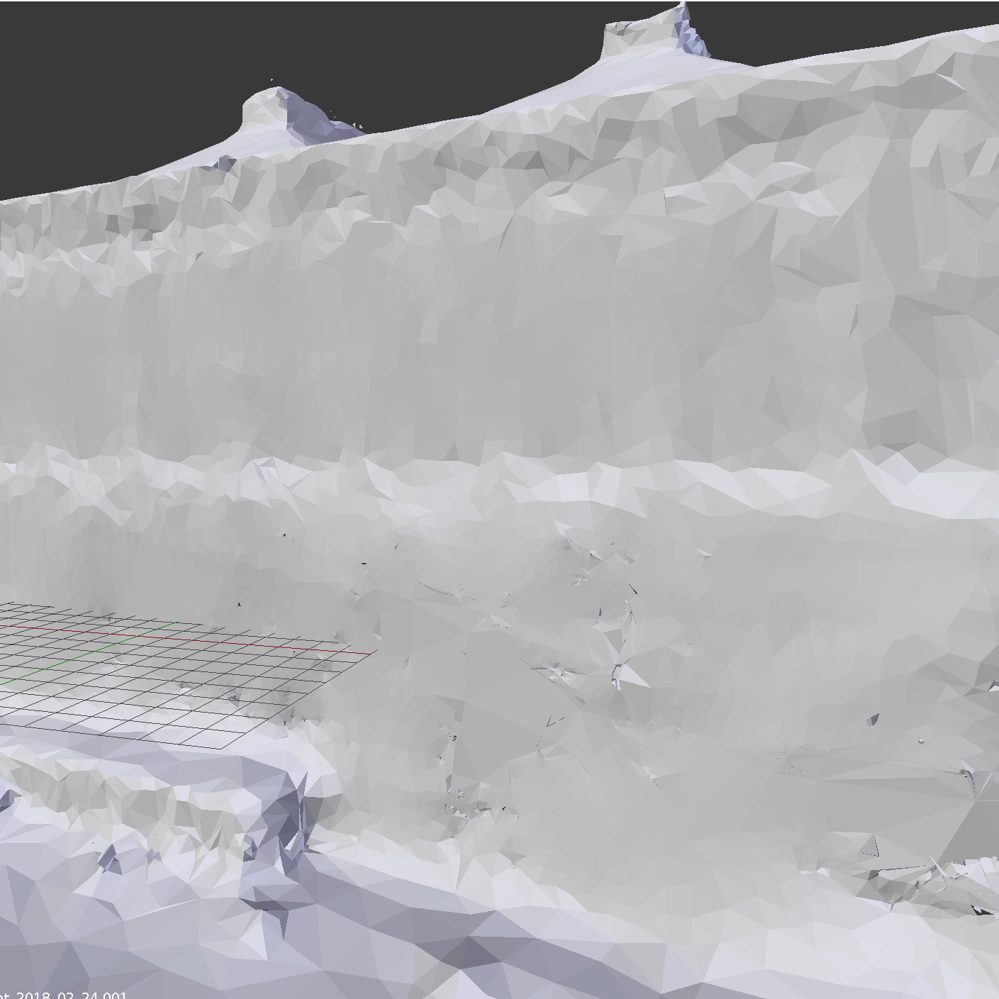
• Go to Tools (left toolbar) ‣ Mesh Tools ‣ Subdivide . The subdivide dialogue should appear on the bottom left on the toolbar. Type 6 in the number of cuts tab.
• Go to 3D view editor's bottom toolbar ‣ Object interaction mode ‣ Object Mode . You should be able to see the surface details at this point (bottom figure, right image).

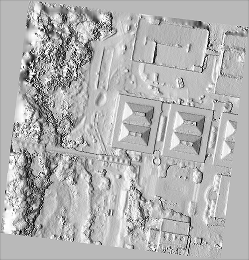
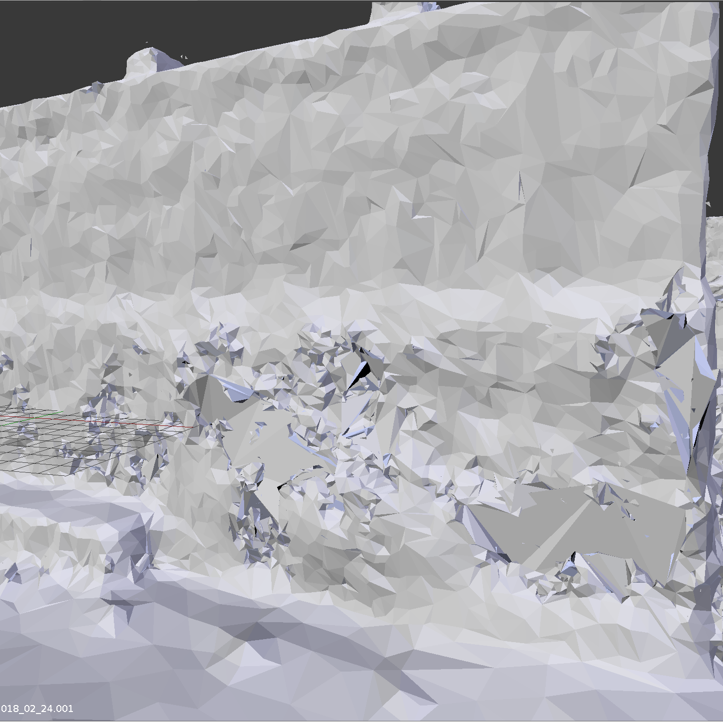
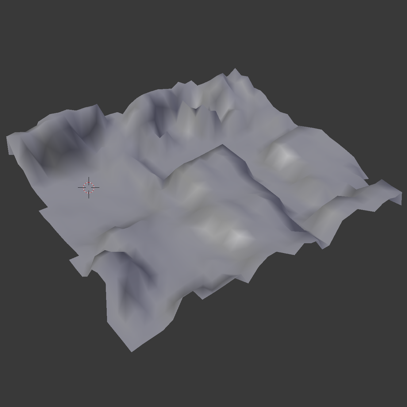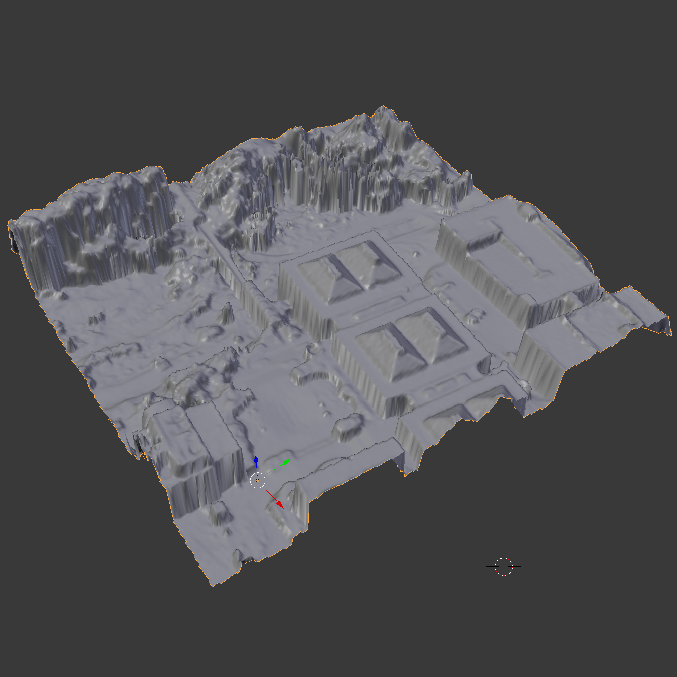DSM surface before subdivision	DSM surface after subdivision

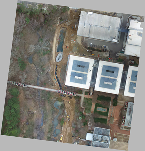
In this step, we juxtapose the DSM and wavefront meshes to compare them.

• Unhide the centennial_OBJ object in the outliner (click on the eye and camera icons).
• Select the centennial_dsm object and press G to grab and move it. You can constrain the movement to each axis by pressing X, Y, Z. Move the object until it is horizontally juxtaposed and vertically aligned with centennial_OBJ object (see figure below).
• Save and close the blender file.

Comparison of wavefront mesh (left) and DSM (right)

---

In the last step, we animate the UAV flight route. First, we lock the Camera object's direction to the center of the UAV model using and "Empty" object and then, we make the camera follow a curve object that represents the flight line.

• Download and unpack the centennial_animation.zip file.

• Open the centennial_animation.blend file.

• To familiarize yourself with Camera :

  • From the outliner select the Camera object. You should be able to see the camera object highlighted in orange (figure).
  • In the viewport bottom headers menu select View > Camera (alternatively you can press numpad 0 to go to camera mode). you should your viewport will change to camera view (see figure).
  • Go to Properties Editor > Camera tab (with the camera icon) to see the camera options.
  • Change with the Focal length to set the field of view.

  
  
  Camera object, flight route object and UAV mesh shown in viewport wireframe mode.

  
  

Since we don't have information about the rotation and tilt of the UAS camera at hand, we assume that it was targeted towards the center of the survey area throughout the flight. This can be done by locking the camera to an "empty" object -- a single coordinate point with no additional geometry -- located at the center of the UAV mesh.

• To create the empty axis:
• In the viewport bottom header menu select Add > Empty > Empty Axis.
• Select the recently added object from outliner.
• Go to Properties Editor > Object (the cube icon) > in the Transform section > change X, Y and Z parameters to 0. This will move the empty axis to the center of the grid.

Adding the Empty object to the scene (left) and moving the empty to 0,0,0 coordinates

• To lock the Camera object to the empty:
  • Select the Camera object in outliner.
  • Go to Properties Editor > Constraints (the chain link icon) > Track to.
  • In the Track to panel set the following parameters (figure):
    • In the Target field select Empty.
    • To parameter to -Z.
    • Up parameter to Y.
• You should be able to see the camera looking towards the empty object.

Track to constraint used to lock the camera to the empty object

• To make the Camera follow the flight_route object:

  • Move camera to the beginning of the flight route line:
    • Select the Camera object and change its X, Y, Z location to 65, -97, 88 (using properties editor's object tab). Alternatively you use G shortcut to freehand move the camera to the tip of the line.
  • Make sure the camera is still selected > Press and hold Shift key and select the flight route object (right-click in the viewport or left-click in the outliner) so that both objects are selected.
  • Press Ctrl + P and select Follow Path.
  • Now the camera follows the path.

  
  
  Set Parent To panel appearing after pressing Ctrl + P while Camera and line object are selected

  
  

• To see the camera following the line:

  • Slide the green line in Time Line editor (the editor below the viewport)to advance the frames (figure below).

  
  
  Camera object follows the flight route curve as timeline slider is moved

  
  

You can render the animation as a video file using the Render tab of the Properties editor (see figure). To render the animation:

• In the Output section define the video output path (e.g., D:/render.avi)
• Press Animation button of the Render section.
• Rendering the animation may take hours to complete as it requires rendering 250 individual frames to create the animation.

Rendering panel