Overview

Trackit is an add-on package for the statistical environment R to efficiently estimate movement parameters and predict "the most probable track" directly from the raw light measurements obtained from archival tagged individuals. Its basic use is to fit and plot the model described in Nielsen and Sibert 2007.

The model is unique in estimating the most probable track without making any light-level threshold assumptions, or constraining the movement of the tag between dawn and dusk. The model generates 2 estimated geographic positions per day (at dawn and dusk) based on light; and 3 estimated positions per day (at dawn, dusk, SST time point) when sea-surface temperature (SST) are used in combination with light. The covariance structure of the model is designed to handle high correlations between light measurements, such as might be caused by local weather conditions. The yearly pattern in latitude precision is estimated by propagating the data uncertainties through the geolocation process. The model has been applied to simulated data, mooring studies, and real deployments on swimming and diving fish.

Publications

• Trackit with SST - Lam, Chi H., Anders Nielsen, and John R. Sibert, 2010. Incorporating sea-surface temperature to the light-based geolocation model TrackIt. Marine Ecology Progress Series 419:71-84
• Trackit - Nielsen, Anders, and John R. Sibert, 2007. State-space model for light-based tracking of marine animals. Canadian Journal of Fisheries and Aquatic Sciences 64: 1055-1068.

Cheatsheet of Trackit

See an example in R before working on your own dataset

https://github.com/positioning/kalmanfilter/blob/master/test-trackit.r

Now, for your own data:

Input data format

1. Light data

> track
  year month day hour min sec depth light  temp
  2003     9   8    2  32   0  22.5   173 21.75
  2003     9   8    2  33   0  22.5   173 21.75
  2003     9   8    2  34   0  23.0   173 21.75
  2003     9   8    2  35   0  22.5   173 21.75
  2003     9   8    2  36   0  22.0   173 21.75
  2003     9   8    2  37   0  22.0   173 21.75

• depth values can be used for correcting light measurements taken at deeper depths. This is only recommended when detailed, high resolution time series is available. Check documentation for usage

  ?two.layer.depth.corr

2. SST data

> tagsst
  year month day hour min sec sst
  2003     9   8    0   0   0  21.7
  2003     9   9    0   0   0  22.5   
  2003     9  14    0   0   0  24.0
  2003     9  16    0   0   0  21.5
  2003     9  22    0   0   0  22.0
  2003     9  28    0   0   0  22.5

• This daily tag-derived SST data frame doesn't have to be continuous. Include any particular day that you have data for.

Basic Workflow

# Note: delete the hash sign (#) at the beginning to uncomment a line

library(trackit)
data(gmt3); data(deltat); deltat$JDE = with(deltat,JDE(year,month,day))

track<-read.table("datafile.dat", header=TRUE) # change file name and path for your own file

prep.track<-prepit(track, fix.first=c(360-161.45,22.85,2002,9,10,0,0,0), 
                   fix.last=c(360-159.87,21.95,2003,5,21,0,0,0), scan=FALSE)

fit<-trackit(prep.track)

1. Load packages

2. Read in data files (light, SST data)

3. (Optional) Perform depth correction of light measurements

  track <- two.layer.depth.corr(track)

4. (Optional) Download SST satellite imagery

  sstfolder <- get.sst.from.server(track,200,250,10,40)
  # the arguments above are the track and bounding box for downloading SST, which is:
  # longitude start, longitude end, latitude start, latitude end
  # longitude is in 0-360 degree system
  
  # Look for help for get.blended.sst if you want to use higher-resolution imagery
  ?get.blended.sst

5. Prepare data for trackit via the prepit function

• Make sure fix.first and fix.last contain the correct release and reporting/ recapture postions
• fix.first or fix.last are formated as below:

(longitude in 0-360 degree system, latitude, year, month, day, hour, minute, second)

• Set scan=FALSE when transmitted light data are used (Wildlife Computer tags)
• Arguments sst and localsstfolder are only required when you desire to do SST matching as well, e.g.

  # Will not run
  # prep.track <- prepit(track, ...,
  #                       sst=tagsst, 
  #                       localsstfolder="c:/temp/sstfolder")

6. Run the model via the trackit function

• It is not uncommon that model fails to converge. Try using different initial values or turn off estimation of some parameters to simplify the model. For instance, for tracks with a very short deployment, try. Here's a table of other tips, thank you Dr Kevin Weng for summarizing it.

  fit <- trackit(prep.track, ss3.ph=-1)

  Tips: other options to use: 
  D.ph=2 or 4, D.i=400 or 1200, 
  ss1.ph=4 or ss2.ph=4 (don't turn off ss1 or ss2, you can but you must check the outputs)
  When SST is used, the parameters rad, bsst and sssst can be tweaked too.

7. Re-run the model where necessary (sorry - this is usually the case!)

• When a model fails to converge, no output files can be generated, and that usually results in a series of warning and error messages. Those messages do not mean there is any software problem other than the model fails (I know, still disappointing). This is a simple of such messages. Return to Step 6 to give it another try.

### An example ###

Error in file(file, "rt") : cannot open the connection In addition:
Warning messages:
1: In dir.create(dirname) :
  'C:\Temp\RtmpEhPlmirun' already exists
2: running command 'C:\Windows\system32\cmd.exe /c ukf.exe' had status 1
3: In shell(cmd, invisible = TRUE) :
  'ukf.exe' execution failed with error code 1
4: In file(file, "rt") :
  cannot open file 'ukf.std': No such file or directory

Subsampling light data

Transmitted light data

• Only available now with Wildlife Computer PSATs
• Light values are already depth-corrected on board of the instrument

Recovered light data time series

• Nielsen and Sibert (2007) show that tracks can be reconstructed with high fidelty even when the time series data are at a lower sampling frequency (up to 14 min between successive observations).
• Sub-sampling full resolution time series will also shorten computation time
• If you want to depth-correct your light measurements, make sure you perform that before sub-sampling your time series
• Sub-sampling can be done with code like below:

  track2 <- track[seq(1,nrow(track),2),] # Retain every other row

Output and Plotting

The fit object

• Although you are free to assign any object for the model output, we use fit consistently throughout to maintain clarity.
• fit is only generated when the model converges. If you see any "Error" messages on the R window, it means the model did not converge and you should re-run the model

> fit
# Trackit version: 0.2-68 
# Date: 23 Aug 2012 (21:03:56) 
# Negative log likelihood: 29322.5 
# Maximum gradient component: 0.0001 
# which means the convergence criteria is obtained.

• You can expose the sub-items in the fit object using the dollar sign operator $

  Parameters:
                D        ss1     ss2     ss3       rho     bsst  sssst
Estimates: 877.62 3.1820e-07 626.920 3.83390 0.0909640 -1.99820 4.9433
Std. dev.: 242.50 9.7674e-05  51.969 0.28756 0.0081853  0.20575 0.6466
                  rad       phi1       phi2    phi3    phi4    phi5    phi6
Estimates: 1.2000e+03 6.0947e-06 4.5281e-06 32.9460 30.5620 35.9190 29.0080
Std. dev.: 8.8795e-03 8.5923e-02 6.4986e-02  4.3112  3.4253  1.2348  1.2637
               phi7   phi8    phi9  phi10      phi11      phi12      phi13
Estimates: 14.75900 6.7251 4.01730 3.4835 1.3194e-08 2.0617e-08 3.1839e-08
Std. dev.:  0.91336 1.0549 0.93292 1.1014 1.9323e-04 2.9227e-04 4.5097e-04
             phi14    phi15
Estimates:  4.6925  0.82745
Std. dev.: 13.5800 29.58500

# This object contains the following sub-items:
 [1] "init"                "phase"               "decimal.date"       
 [4] "sstobs"              "most.prob.sst"       "date"               
 [7] "timeAL"              "most.prob.track"     "var.most.prob.track"
[10] "est"                 "sd"                  "npar"               
[13] "nlogL"               "max.grad.comp"      

# To access these items use the $ operator. For instance
# to get the most probable track type: fit$most.prob.track

Number of estimated positions

• fit$most.prob.track will give you 2 estimated geographic positions per day (at dawn and dusk) based on light; and 3 estimated positions per day (at dawn, dusk, SST time point) when sea-surface temperature (SST) are used in combination with light

Diagnosis: plot function

• Plot of longitude, latitude, and SST (if used) time series can be shown with the command:

  plot(fit)

• Confidence regions are shown in lilac and data points are plotted as crosses

Mapping: fitmap function

• Built-in mapping allows quick visualization of fitted track. To call,

  fitmap(fit, ci=T) # ci = T turns on the confidence regions
  points(fit$most.prob.track, pch=20, col="black") # plot waypoints

A fix for animals crossing from 360 to 0 longitude and vice versa

The following table summarizes whether this fix is needed, when an animal at some point at liberty has crossed (or go back and forth between) the 0/360 longitude line:

Starting longitude (deployment)	Ending longitude (popoff/ recovery)	Fix needed	Notes
West, e.g., 70 W	East, e.g., 10 E	Yes
East, e.g., 10 E	West, e.g., 70 W	Yes
West, e.g., 70 W	West, e.g., 40 W	No	Only the SST step is needed if running Trackit+SST
East, e.g., 10 E	East, e.g., 5 E	No	Only the SST step is needed if running Trackit+SST

SST step (for running Trackit+SST) - just make sure you download all data from 0-360 longitude

### For example, we are requesting all data between 26 and 51 N for the world
  
sst.path<-get.sst.from.server(track, lonlow=0, lonhigh=360, latlow=26, lathigh=51)

1. Download a hotfix script

require(trackit); require(devtools)
source_url('https://github.com/positioning/kalmanfilter/raw/master/support/trackit/lon180trackit.r')

2. Obtain simulated example files for a migratory bird (start West, end East) to follow along

### Simple function to download text files through https
read.txt <- function(url, sep=' ', head=T,...){
  require(httr)
  lfile <- paste(tempdir(),'txtfile.txt',sep='/')
  writeBin(content(GET(url), "raw"), lfile)
  return(read.table(lfile, sep=sep, head=head, ...))
}

### Reading the test files
track <- read.txt("https://github.com/positioning/kalmanfilter/raw/master/testdir/180case/light.dat")
sst <- read.txt("https://github.com/positioning/kalmanfilter/raw/master/testdir/180case/sstvalues.csv", sep=",")
truth <- read.txt("https://github.com/positioning/kalmanfilter/raw/master/testdir/180case/truth.dat", head=F)


### No SST values when the bird went over land
sst <- subset(sst, sst>0)

3. Run prepit as usual

### Running Trackit+SST, therefore, download the satellite imagery
sst.path = get.sst.from.server(track,0,360,26,51)
  
### prepit step
prep.track<-prepit(track, sst=sst, 
                   fix.first=c(285,35,2003,1,1,0,0,0),
       			   fix.last=c(10.96376520823528721849,35.92527349625796517785,2004,1,1,0,0,0))  

4. Apply the hot fix and run trackit as usual

### Direction: "WE" for West to East, otherwise "EW" for East to West
prep.track <- hotfix.dayline(prep.track, direction="WE") 
  
fit <- trackit(prep.track, rad.ph=-1, D.i=1200, rad.i=400)  

5. Adjust longitude values from 0-360 to -180 to 180 for plotting purposes

fit <- switch2lon180(fit)
  
### Plotting
fitmap(fit, ci=T)
points(truth, cex=.6)
points(fit$most.prob.track, col=2,pch=20)  # Trackit solution in red points

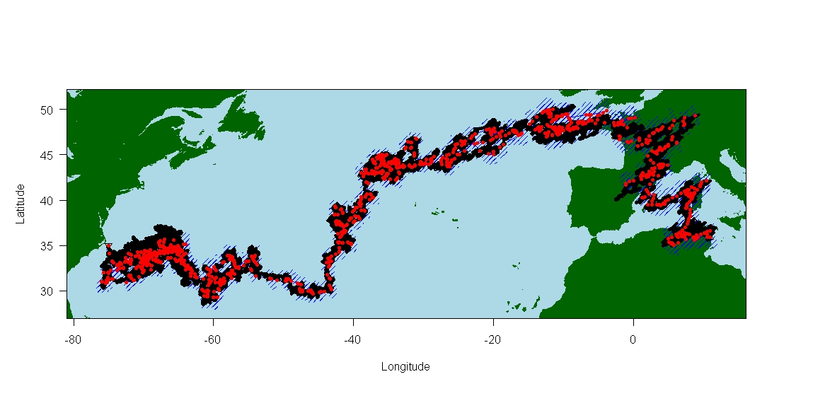
And finally the results,

# Trackit version: 0.2-6 
# Date: 25 Jun 2014 (10:05:46) 
# Negative log likelihood: 27232 
# Maximum gradient component: 0.0012 
# which does not meet the convergence criteria, 
# but is very close, so convercence so is likely 
# obtained anyway.

Parameters:
                  D        ss1      ss2      ss3       rho    sssst     phi1   phi2     phi3      phi4      phi5      phi6
Estimates: 1335.600 3.0727e-07 0.354900 2.396500 0.0078059 0.353690 50.72500 12.942 14.52500 15.080000 13.952000 12.153000
Std. dev.:   70.712 6.5068e-06 0.059006 0.065179 0.0021121 0.033441  0.59735  0.531  0.15059  0.098347  0.085629  0.086508
              phi7     phi8     phi9    phi10    phi11   phi12   phi13   phi14  phi15
Estimates: 9.08010 6.378500 4.841200 3.701200 2.995100 2.42930 2.18620 1.59080 2.4640
Std. dev.: 0.08626 0.084381 0.082508 0.084133 0.088606 0.10076 0.12504 0.18936 0.6043

Troubleshooting for R-3.0+

R-3.0 has made some changes to their base functions, and whenever their team decided to do that, they screw us up. Here are fixes we can find after plenty of hard work of tracking them down

• Missing data When it happens - trying to call fitmap( ) to plot the data on a map

  # Fix: load the data before plotting
  data(gmt3)

• Error in table When it happens - trying to call prepit( ) and is presented with an error

  # Error message: Error in table$JDE: object of type 'closure' is not subsettable

  # Fix: load the data before calling prepit()
  data(deltat); deltat$JDE = with(deltat,JDE(year,month,day))
  

Known issues

1. Light data must have a continuous sinusoidal-like waveform, i.e. light "curves" that function resemble square waves (box-car) will not work well in Trackit. Tags that uses the light sensors as an "on-off" switch will not provide adequate information for Trackit to run, which includes recovered tags from Microwave Telemetry and bird tags from BAS.