The geometry domain

Motivation

3 different styles that give insight into the math
Broadly accessible and useful domain
Deeply linked to the history and origins of math (Euclid's axioms and parallel postulate) as well as the meaning of math (Hilbert on abstraction)
Lots of comparison libraries for evaluation
Can deploy the domain, e.g. to create the illustrated Euclid's elements
Makes for a great teaser figure

Domain files: https://github.com/penrose/penrose/tree/geometry/src/geometry-domain

Euclidean style

runpenrose geometry-domain/teaser.sub geometry-domain/euclidean.sty geometry-domain/geometry.dsl

TODO

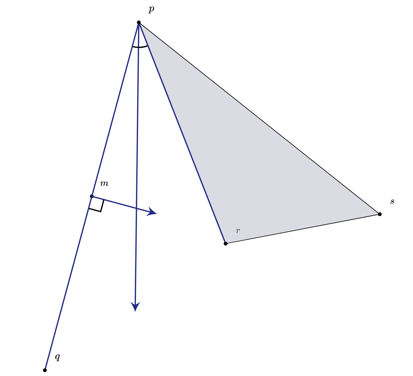
Calculate angle bisector
Clean up code with 2-tuples
Draw bisector angle mark
Labels

Spherical style

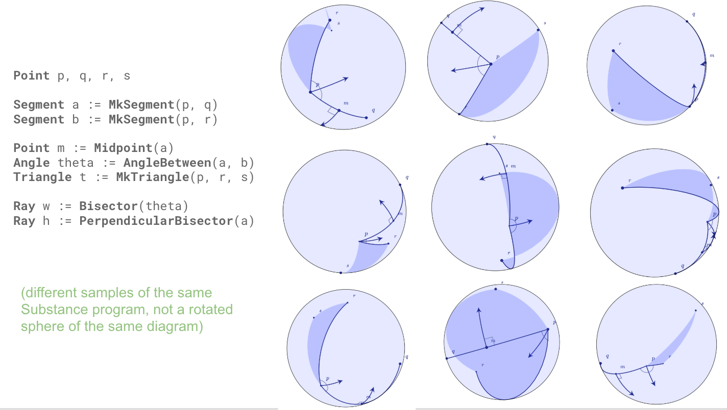
runpenrose geometry-domain/teaser.sub geometry-domain/spherical.sty geometry-domain/geometry.dsl

TODO

drastically improve labeling
make diagram look more 3D (e.g. visibility tests, shadows)
more general renderer

Hyperbolic style

We draw in the Poincare disk model. A point lies on the hyperboloid of two sheets: x^2 + y^2 - z^2 = -1, where z > 0. That is, <p, p>_L = 1 (where <., .>_L denotes the Lorenz inner product).

The overall approach here is very close to that of measuring quantities on a sphere using geodesics.

To draw a point on the hyperboloid, we construct a point that satisfies the hyperboloid by construction: the x and y coordinate are varying, and the z coordinate is calculated to lie on the hyperboloid. Then, since the points that are sampled are liable to look like ideal points (because x and y are much larger than one, we optimize the norm squared of [x,y] to be less than some constant (currently 5).

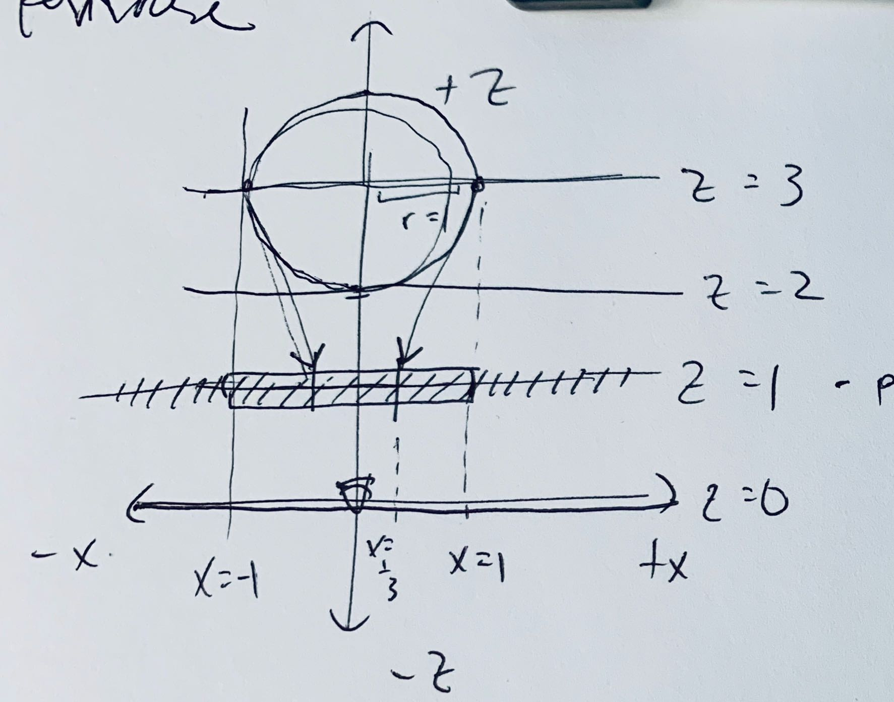
Then we project the point on the hyperboloid into screen space as follows:

project it onto the Poincare disk: [x, y, z] |-> [x / (z + 1), y / (z + 1)]
convert from math space to screen space by multiplying [x, y] by a constant (currently 200)

To understand a vector on the hyperboloid, imagine the line from the origin to the point on the hyperboloid in R^2.

To draw a geodesic (shortest path) between two points, it's very similar to the sphere. Basically we "slice" the hyperboloid in their shared plane and use an arc-length parametrization to walk the hyperboloid along that slice.

Denote the Lorenz inner product x1y1 + x2y2 - x3y3 as <x, y>L.
Assuming a and b lie on the hyperboloid (x^2 + y^2 - z^2 = -1, z > 0)
For a vector v on the hyperboloid, <v, v>L = -1
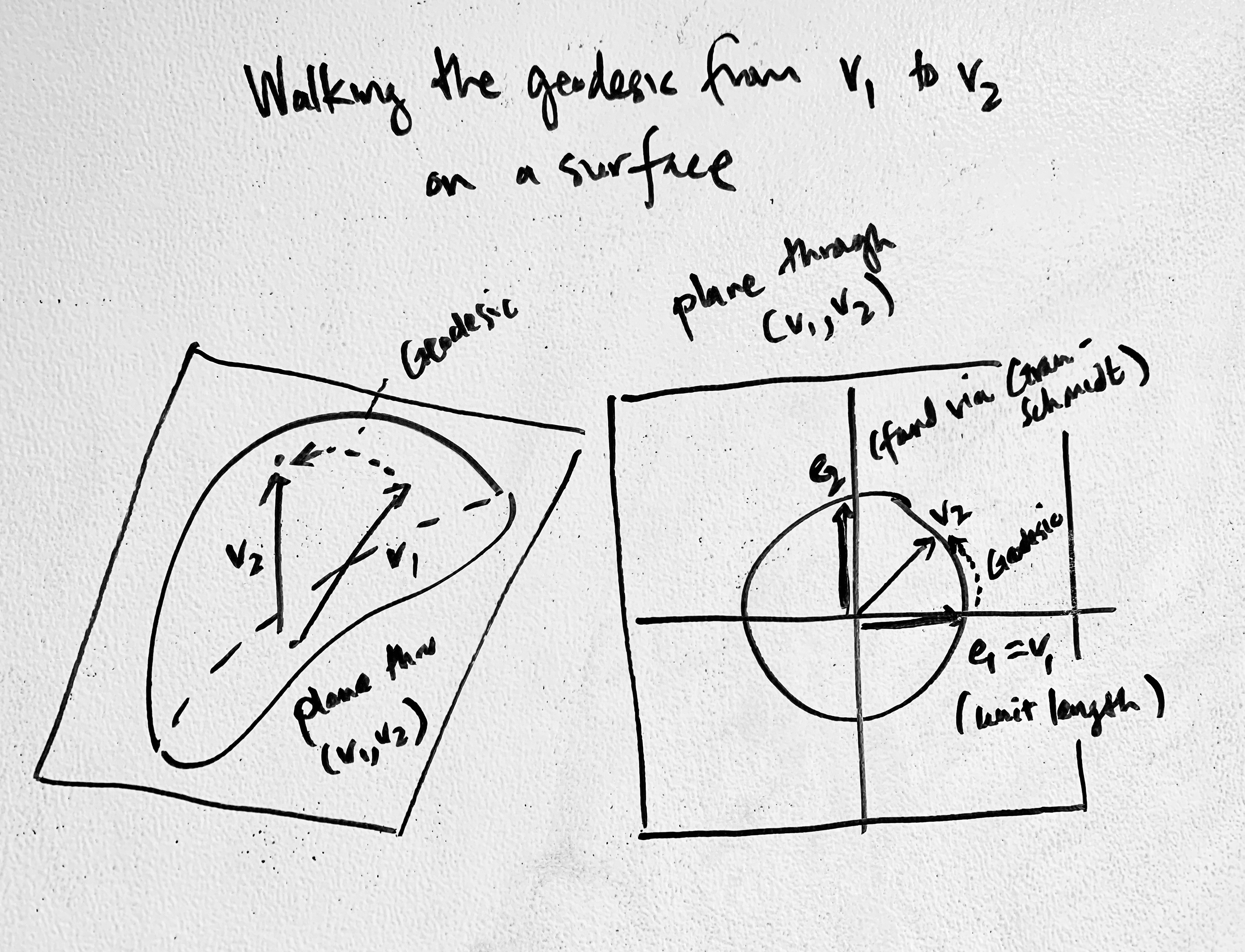
If we start with two vectors a, b on the hyperboloid, then we find an orthonormal basis for the plane that they span by using Gram-Schmidt:
- e1 = a
- e2 = normalize(b + <a, b>L * a)
- (note the sign change: b + proj_a(b), NOT -)
e2 is the unit tangent vector at a in the direction of b. (This is a general method for finding that tangent vector)
(See the picture on the blackboard)
Then we walk starting at a to b, using e1 cosh d + e2 sinh d, where d is the hyperbolic distance between a and b

To draw a triangle, we draw three geodesics.

To draw a perpendicular bisector of a geodesic, we first walk halfway along the geodesic. Then, we turn 90 degrees and walk by some length in that direction. To turn 90 degrees, we can just use the Lorenz cross product (which just changes the sign of the last element of a normal cross product), normalized.

To draw a perpendicular mark, this is actually a little tricky because the mark needs to look perpendicular in 2D space, so we actually walk along the two "legs" of the perpendicular rays in hyperboloid space, project them into screen space, and then draw the perpendicular mark in screen space.

To find the tangent plane at a point on the hyperboloid: note that the tangent plane is defined by two basis vectors (e1, e2) at a point p. To find those two basis vectors, given two other points q and r on the hyperboloid:

Find the tangent vectors tq and tr toward each of those points via hyperbolic Gram-Schmidt (which yields a vector in the plane of each of those points).
Then the first basis vector is either tangent vector, you can Lorentz-cross-product the tangents to get a normal, then Lorentz-cross-product the first two again to get the second (orthogonal) basis vector.

Note that using those basis vectors to walk a geodesic will move from e1 toward e2.

To measure an angle between two geodesics, given three vectors on the hyperboloid, use the hyperbolic law of cosines. (Not sure why the implementation required two legs of the triangle to be equal)

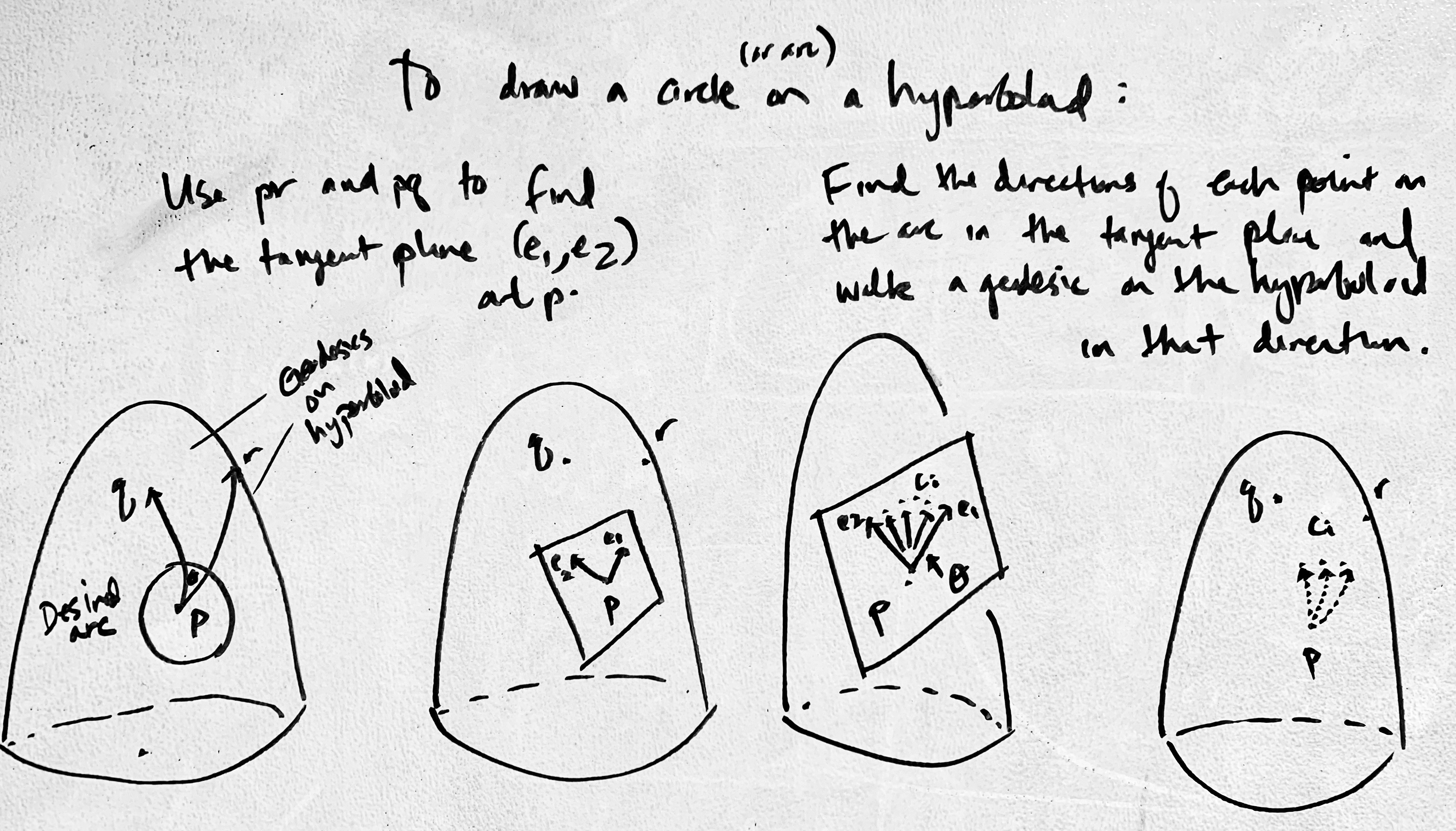
To draw an arc of a circle centered at a point (e.g. angle mark),

Given the basis (e1, e2) (found via the hyperbolic Gram-Schmidt procedure earlier), we can get a vector e in the tangent plane at angle theta from e1 towards e2 by e = e1*cos(theta) + e2*sin(theta). (Maybe you have to normalize here to make sure that it's unit?)
From here, use the arc length parameterized geodesics we have. They say that the point at distance r from P in the direction of the unit tangent vector e is: P * cosh(r) + e * sinh(r)
So, feed e into P*cosh(r) + e*sinh(r) to get the point at radius r and angle theta.
Now vary theta to get your arc.

To draw an angle bisector, use the arc function but just walk halfway.

To draw an angle wedge, also walk along the legs of the angle, but reverse one of the paths.

To label the points via optimization:

For making sure text doesn't overlap curve: first, downsample the curve, then make a repel objective between every point sample and the center of the text bbox
I still use the constraint that places a text box at a distance from a vertex via the signed distance from bbox to point. (So this is NOT point-to-point. It's too hard to get that nice placement with repel and near objectives only, which are imprecise.) I just lowered the padding factor
Pointwise repel between all vertices (not labels, just points) so the diagram looks more spread-out

Note that all curves are generated in hyperbolic space, so points in screen space are going to "bunch" near the ends, which might interfere w/ any pointwise methods; I don't resample the curve uniformly by arc length.

Also everything is still all jointly optimized.

(Another note about repel objectives: they tend to "add up" to extra padding where curves intersect, whereas constraints give better visual results)

Implementation notes:

Note that the distance, norm, angle, dot product, cross product, projection, Gram-Schmidt, etc. all have to be done differently in Lorenz space, and they all have to use the right implementation (flipping the last sign).
To calculate the norm of a vector, take the absolute value before you sqrt, otherwise the norm may be negative (?).

Related docs:

Implementation

This style draws a sphere of radius 1.

The spherical style is implemented by performing spherical geometry operations in 3D Cartesian coordinates (XYZ, not polar coordinates, since polar coordinates are very poorly behaved for optimization) and enforcing that all points on the sphere have norm 1.

An arc on a sphere, between two points p and q on the sphere, is drawn by walking the great circle including those points. This is done by forming an orthonormal basis at p and walking to q. Note that on a unit sphere, the angle between points is the length of the arc between them.

The positions of the camera and sphere in 3D are hardcoded, as is the direction of the camera and the screen transform. The sphere is located at the origin with a radius of 1, and the camera is located at (0, 0, -3) looking down the positive z-axis, so the camera is at a distance of 2 from the sphere.

The diagram is drawn in 2D by doing the following:

Translating in 3D so the camera is at the origin
Doing a perspective projection (mapping (x,y,z) to (x/z, y/z)). After step 1, this divide implicitly projects the sphere on a projective plane z=1. (Note: be careful that the sphere is at a sufficient distance from the projective plane.)
Multiplying by an arbitrary constant to convert from math space to screen space

The diagram below shows the configuration of the objects after step 1.

A point on the sphere is rendered as a circle whose radius is scaled linearly, from the min/max z of the sphere to an arbitrary range such that the radius is larger as the point is closer to the camera.

An arc is rendered by projecting each of its sample points to 2D and creating an open path connecting those points.

Optimization can be performed on the 3D objects or on their projected 2D shapes.