Penrose has a custom system that will automatically calculate gradients of your code. Here is how to use it.

All objectives, constraints, and functions need to be written in a differentiable manner. That means that all numbers need to actually be special types called VarADs that have special ops applied to them, so the system can track what operations are being applied to what, so it can take the gradient for you. (That means you currently can't write something like, say, v + w. Rather, you need to use the add operator.)

You can convert to and from number and VarAD using the convenience functions varOf (or constOf) and numOf. You can also apply atomic and composite operations to VarADs, detailed below. Beyond that, you should not directly modify the VarADs.

In the system, all arguments to objectives/constraints/functions are (should be) automatically converted to VarADs, though if not, you can use the constOfIf function.

You must write your function in a purely functional style, without mutating variables, otherwise the autodiff won't work, because that will create a cycle in the computation graph. Avoid writing something like this to express x = x + 1:

let x = add(x, constOf(1))

Instead, make new constant intermediate variables:

const x0 = ... const x1 = add(x0, constOf(1))

Internally, each operation on VarADs creates a computation graph linking the children and parents of each operation. In Penrose, a computation graph has just one head node -- the overall energy of a diagram. Evaluating a computation graph yields a single scalar value. In practice, you don't have to worry about that.

See contrib/Functions and contrib/Constraints.

Here's an example of a constraint written using the autodiff.

We might want to constrain one circle s1 to be smaller than another circle s2 by some amount offset. In math, we would require that r1 - r2 > offset. An inequality constraint needs to be written in the form p(x) > 0, since we penalize the amount the constraint is greater than 0. So, this constraint is written as r1 - r2 - offset > 0, or p(r1, r2) = r1 - r2 - offset. Let's say we want the offset to be some function of the larger circle's radius, say 0.4 * r2. That penalty is written as the following constraint function:

smallerThan: ([t1, s1]: [string, any], [t2, s2]: [string, any]) => {
  // s1 is smaller than s2
  const offset = mul(varOf(0.4), s2.r.contents);
  return sub(sub(s1.r.contents, s2.r.contents), offset);
}

All operations are defined in engine/Autodiff.ts. For documentation of their type signatures, see this autogenerated page for the module.

Atomic operations supported:

• Unary
  • sin
  • cos
  • neg
  • squared
  • absVal
  • sqrt
  • inverse
• Binary
  • add
  • mul
  • sub
  • div
  • max
  • min
  • gt
  • lt
• Trinary
  • ifCond
• N-ary
  • addN

Composite operations (in ops), on vectors (VarAD[]) or multiple VarADs

• norm (two variables)
• dist (two variables)
• vadd
• vsub
• vnormsq
• vnorm
• vmul
• vdiv
• vnormalize
• vdist
• vdistsq
• vdot
• vsum

Additional vector helper functions are available in OtherUtils.

Helper functions

• toPenalty
• center

Since energies and gradients are compiled into bare-bones JS code, any console.log you put in your function definitions will not result in output during the optimization (since it doesn't show up in the computational graph for the energy).

However, we provide a function that has an equivalent effect, called debug. It behaves functionally, not imperatively. That is, you can pass it a node and (optionally) a debug string to print, and it returns a node that you should use as usual in the computational graph that you're building up in an energy/constraint/function. (If you don't use that returned node, no debug output will show up, so this is not an imperative log-type statement.)

For example, let's say we're working with this program triple:

runpenrose set-theory-domain/tree.sub set-theory-domain/tree.sty set-theory-domain/setTheory.dsl

To print some quantities in the objective centerArrow, we wrapped some variables in debug as below:

  centerArrow: ([t1, arr]: [string, any], [t2, text1]: [string, any], [t3, text2]: [string, any]): VarAD => {
    const spacing = debug(varOf(1.1)); // NOTE: used to be just `varOf(1.1)`

    if (typesAre([t1, t2, t3], ["Arrow", "Text", "Text"])) {
      const c = mul(spacing, text1.h.contents);

      return centerArrow2(arr, fns.center(text1), fns.center(text2),
        [debug(c, "c from centerArrow"), // NOTE: used to be just `mul(spacing, text1.h.contents)`
        neg(mul(text2.h.contents, spacing))]);

    }

Then, the debug output will come every time the relevant variable's value is calculated in either the energy or the gradient. For example, since in this triple of programs to make a tree diagram, the centerArrow objective is applied six times (once to each while), it results in six energy debug statements per quantity (times two quantities, spacing and c), and six gradient debug statements per quantity (times two quantities).

VM16989:473 no additional info (var x508) | value:  1.1 during energy evaluation
VM16989:476 c from centerArrow (var x510) | value:  13.200000000000001 during energy evaluation
VM16989:525 no additional info (var x558) | value:  1.1 during energy evaluation
VM16989:528 c from centerArrow (var x560) | value:  13.750000000000002 during energy evaluation
VM16989:576 no additional info (var x607) | value:  1.1 during energy evaluation
VM16989:579 c from centerArrow (var x609) | value:  13.200000000000001 during energy evaluation
VM16989:627 no additional info (var x656) | value:  1.1 during energy evaluation
VM16989:630 c from centerArrow (var x658) | value:  13.200000000000001 during energy evaluation
VM16989:678 no additional info (var x705) | value:  1.1 during energy evaluation
VM16989:681 c from centerArrow (var x707) | value:  13.200000000000001 during energy evaluation
VM16989:729 no additional info (var x754) | value:  1.1 during energy evaluation
VM16989:732 c from centerArrow (var x756) | value:  13.750000000000002 during energy evaluation

VM16990:463 no additional info (var x498) | value:  1.1 during grad evaluation
VM16990:466 c from centerArrow (var x500) | value:  13.200000000000001 during grad evaluation
VM16990:612 no additional info (var x645) | value:  1.1 during grad evaluation
VM16990:615 c from centerArrow (var x647) | value:  13.750000000000002 during grad evaluation
VM16990:1175 no additional info (var x1206) | value:  1.1 during grad evaluation
VM16990:1178 c from centerArrow (var x1208) | value:  13.200000000000001 during grad evaluation
VM16990:1322 no additional info (var x1351) | value:  1.1 during grad evaluation
VM16990:1325 c from centerArrow (var x1353) | value:  13.200000000000001 during grad evaluation
VM16990:1833 no additional info (var x1860) | value:  1.1 during grad evaluation
VM16990:1836 c from centerArrow (var x1862) | value:  13.200000000000001 during grad evaluation
VM16990:1980 no additional info (var x2005) | value:  1.1 during grad evaluation
VM16990:1983 c from centerArrow (var x2007) | value:  13.750000000000002 during grad evaluation

For debugging purposes, derivatives of any variable are available in Style. This way, you can (say) visualize the direction the optimizer thinks it should move some object in order to decrease the energy / satisfy the constraints. You can access derivative(x) or derivativePreconditioned(x), where x is any varying variable, derivative returns ∂F/∂x, and derivativePreconditioned returns the preconditioned descent direction for that variable. E.g., we currently apply L-BFGS to get the actual descent direction.

To use this, you'll have to set DEBUG_GRAD_DESCENT in engine/Optimizer.ts to true (because gradient information is only received once per display step, and this setting lowers the number of optimization steps per display step).

Here is an example, where the derivative of text position shown in red, and preconditioned derivative shown in blue:

runpenrose set-theory-domain/twosets-simple.sub set-theory-domain/venn-small.sty set-theory-domain/setTheory.dsl

(derivative of text position shown in red, preconditioned derivative shown in blue)

Style: (note the two debug arrows)

forall Set x {
    x.shape = Circle {
        x : ?
        y : ?
        r : ?
        -- r : 100.0
        strokeWidth : 0
    }

    x.text = Text {
        string : x.label
    }

    LOCAL.c = 20.0

    x.debugShape = Arrow {
        startX: x.text.x
        startY: x.text.y
        endX: x.text.x + LOCAL.c * derivative(x.text.x)
        endY: x.text.y + LOCAL.c * derivative(x.text.y)
        color: rgba(1.0, 0.0, 0.0, 0.5)
        arrowheadSize: 0.5
        thickness: 3.0
        style: "dashed"
    }

    LOCAL.d = 20.0

    x.debugShape2 = Arrow {
        startX: x.text.x
        startY: x.text.y
        endX: x.text.x + LOCAL.d * derivativePreconditioned(x.text.x)
        endY: x.text.y + LOCAL.d * derivativePreconditioned(x.text.y)
        color: rgba(0.0, 0.0, 1.0, 0.5)
        arrowheadSize: 0.5
        thickness: 3.0
        style: "dashed"
    }

    ensure contains(x.shape, x.text) -- NEW
    encourage sameCenter(x.text, x.shape) -- OLD

    ensure minSize(x.shape)
    ensure maxSize(x.shape)
}

A computation graph is a directed acyclic graph (DAG) of the atomic operations involved in computing a function. It contains nodes and edges.

A node in the graph is either a varying variable (like v), a constant (like 1.0), or an operation (like mul(v,w)) on nodes. Nodes have type VarAD.

A computation graph can model either the energy (referred to as the energy graph) or the gradient (referred to as the gradient graph).

An edge (from child to parent) in an energy graph is a sensitivity.

Let's say we wanted to add a operation and its gradient to the autodiff. We'll take mul(v,w) as an example (which just multiplies two numbers). Here are the steps.

1. Add a new top-level definition of the operation, and its gradient in Autodiff

Let's denote the parent node, mul(v,w), as z. It has two children, or inputs, v, and w. In the computation graph, we have to create edges (pointers) from z to its two children v and w, as well as pointers from each child to its parents. (This is because we need to traverse the graph "bottom-up", from child-to-parent, to perform the reverse-mode autodiff, and we need to traverse the graph "top-down," from parent-to-child, to evaluate the graph's energy.)

Not only that, but a quantity lives on the edge from each child to its parent, called a "sensitivity." "Sensitivity" just means how much changing an input a little affects the output. Here it's the partial derivative: the sensitivity from v to z is dz/dv in general, which in this context is d mul(v,w)/dv = w.

     s ("single output" node)
    ...
    PARENT node (z) -- has refs to its parents
     ^
     | sensitivity (dz/dv)
     |
    var (v)         -- has refs to its parents
(carries gradVal: ds/dv)

(TODO: Put in a real diagram.) (I'm glossing over some mathematical details here, this is not quite what a sensitivity is, but check out this post for a more detailed explanation.)

In our system, a VarAD can either be an energy node (i.e. it lives in the computation graph of an energy) or a gradient node (i.e. it lives in the computation graph of the gradient). They are distinguished by the boolean parameter isCompNode.

An edge between energy nodes (VarAD) can carry a gradient function, which is a sensitivityNode. The sensitivityNode is a VarAD itself, or a fragment of a computational graph, linked to gradient and energy nodes.

We know that grad mul(v,w) = [w, v]. So, in both the energy graph and the gradient graph, we want to set z's children to be w and v, and v and w's parent's to be z. Only in the energy graph, do we store the sensitivities, that is, the sensitivityNode from v to z should be just(w), like the partial derivative (and likewise for w).

We also store the op of the node, which below is *. This string is used by default in the code generation.

export const mul = (v: VarAD, w: VarAD, isCompNode = true): VarAD => {
  const z = variableAD(v.val * w.val, "*"); // Initialize the node with the value applied to the childrens' values now -- this isn't really used in the graph
  z.isCompNode = isCompNode; // Need to add this line in case `mul` shows up in a gradient ntode

  if (isCompNode) { //
    v.parents.push({ node: z, sensitivityNode: just(w) });
    w.parents.push({ node: z, sensitivityNode: just(v) });

    z.children.push({ node: v, sensitivityNode: just(w) });
    z.children.push({ node: w, sensitivityNode: just(v) });
  } else {
    v.parentsGrad.push({ node: z, sensitivityNode: none });
    w.parentsGrad.push({ node: z, sensitivityNode: none });

    z.childrenGrad.push({ node: v, sensitivityNode: none });
    z.childrenGrad.push({ node: w, sensitivityNode: none });
  }

  return z;
};

In general you will need to define and cache sensitivity nodes, making sure all quantities involved are gradient nodes. Here is a more complicated example of adding a discontinuous atomic operation.

export const max = (v: VarAD, w: VarAD, isCompNode = true): VarAD => {
  const z = variableAD(Math.max(v.val, w.val), "max");
  z.isCompNode = isCompNode;

  const cond = gt(v, w, false);

  // v > w ? 1.0 : 0.0;
  const vNode = ifCond(cond, gvarOf(1.0), gvarOf(0.0), false);
  // v > w ? 0.0 : 1.0;
  const wNode = ifCond(cond, gvarOf(0.0), gvarOf(1.0), false);

  // NOTE: this adds a conditional to the computational graph itself, so the sensitivities change based on the input values
  // Note also the closure attached to each sensitivityFn, which has references to v and w (which have references to their values)

  if (isCompNode) {
    v.parents.push({ node: z, sensitivityNode: just(vNode) });
    w.parents.push({ node: z, sensitivityNode: just(wNode) });

    z.children.push({ node: v, sensitivityNode: just(vNode) });
    z.children.push({ node: w, sensitivityNode: just(wNode) });
  } else {
    v.parentsGrad.push({ node: z, sensitivityNode: none });
    w.parentsGrad.push({ node: z, sensitivityNode: none });

    z.childrenGrad.push({ node: v, sensitivityNode: none });
    z.childrenGrad.push({ node: w, sensitivityNode: none });
  }

  return z;
};

2. Check the arity of the operation and add the appropriate code generation (to JS) in traverseGraph

In traverseGraph, you should define how your operation is translated into JS code, which is just a string with the appropriate parameters. For mul, since we set the node's op to be *, that's what's used by default in the code generation:

stmt = `const ${parName} = ${childName0} ${op} ${childName1};

But you can also define custom code that should be emitted, such as the more complicated example of an n-ary addition:

if (op === "+ list") {
  const childList = "[".concat(childNames.join(", ")).concat("]");
  stmt = `const ${parName} = ${childList}.reduce((x, y) => x + y);`;
}

Add it to ops as in this example:

  vnormalize: (v: VarAD[]): VarAD[] => {
    const vsize = add(ops.vnorm(v), varOf(EPS_DENOM));
    return ops.vdiv(v, vsize);
  },

There's no need to add a gradient, codegen, etc.

To find small example computation graphs, as well as unit tests for them, look at testGradSymbolicAll.

The module also includes a function, testGradSymbolic that tests the autodiffed gradient of a function by checking it against the gradient computed via finite differences. It is very useful for checking that the custom analytic gradient of a new operation is correct.

(TODO: Currently the finite difference tests will "fail" if the gradient magnitudes are greater than eqList's sensitivity, when really it's fine. Fix this.)

• Mutable state
• For-loops
• Optimizations on the computation graph
• Detecting cycles in the computation graph
• Matrix/tensor ops or derivatives at leaves
• Higher-order derivatives, like Hessians
• Visualizing the energy or gradient graph

• Sometimes the codegen will loop forever. This is probably because there is a cycle in the graph. (TODO: prevent this)

Short answer: We already tried. Those systems are optimized to perform operations on huge tensors, small computation graphs. Our system has a lot of operations on single scalars, with a relatively deep computational graph. Therefore the overhead is in the interpretation, not (say) matrix multiplies. That's why we wrote our own system.

First, a little bit about various approaches to autodiff (AD). It's all basically the chain rule, the question is just in what order and when to apply it.

On ordering:

Forward mode AD applies the operator d./dxi recursively from the top down. That means any intermediate results are only about that particular dependent variable xi. So, forward-mode AD is good for a computational graph with one input and many outputs. Forward-mode AD is also really simple to implement with a typeclass.

Reverse mode applies the operator dz/d. from the bottom up, also recursively. That means it generates the partial derivative with respect to intermediate nodes. So any intermediate results are not tied to a particular dependent variable, but to the intermediate node, and can be reused for any of its children, because you are changing the dependent variable. This is the approach we want to use, since our energies have many inputs and one output.

On timing:

Regardless of mode, AD can also be performed at different stages of the computation process. It can be done dynamically or statically. Dynamically means that the graph is built and the energy is evaluated as the computation itself is executed--this is known as the "forward pass"--then the gradients are taken at runtime on the graph you just built, known as the "backward pass." An alternative is to transform the energy graph into a gradient graph, then compile the gradient graph into code. This is the approach we take, which I call "static" because it is executing native code in the host language.

Example. Here's a short example illustrating reverse-mode AD on a graph.

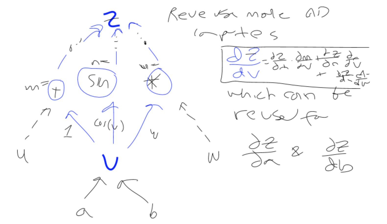
We want to calculate the partial derivative of the head node, z, with respect to any intermediate node v (not necessarily a leaf node, though in practice we start from the leaves). That is dz/dv. To do that, we realize that v could have been used in several operations that might be influencing the output z, i.e. that v might have several parents, p_i. We want to figure out how much changing v influences its parents, which influence z. So, we apply the chain rule to sum the partial derivatives over v's parents, which are then calculated recursively to find out how much each of v's parents is influencing z.

In normal notation: dz/dv = \sum_{i=1}^n dz/d(p_i) * dp_i/dv

In function notation: dz/d(v) = \sum_{i=1}^n dz/d(p_i) * dp_i/dv

(where dz/d(.) is the function that's being applied recursively)

dpi/dv is the sensitivity (a function that lives on each of the edges from the current node, v, to each of its parents, m, n, and o--yes, that's an o). In the picture above, two sample sensitivities (between v and its parents p_1 and p_2) are:

dp_1/dv = dn/dv = cos(v)
dp_2/dv = do/dv = w

Implementation:

The function that actually takes the gradient symbolically is called gradAllSymbolic. It performs reverse-mode autodiff symbolically, which means that given a computational graph of the energy function, it returns a computational graph of the gradient.

It does this by going "bottom-up," i.e. starting with all the leaf variables that marked as changeable, that we're taking the gradient with respect to. Then, it applies exactly the math discussed above, but instead of computing the partial derivative, it builds a gradient graph describing the partial derivative, and stores the resulting pointer in the node, to be turned into code later.

The main code is just one line:

const gradNode: VarAD = addN(v.parents.map(parent =>
  mul(fromJust(parent.sensitivityNode), gradADSymbolic(parent.node), false)),
  false);

After running this function, each leaf node v has the node of dz/dv stored in its gradNode property.

Note that evaluating the gradient depends on evaluating the energy, so the graphs' nodes may be linked, i.e. that some gradNodes may include pointers to node in the energy graph.

For a more detailed explanation, see this blog post and this one.

Then, both the energy graph and gradient graph are compiled into code, which is constructed at runtime and hopefully JITted by the JS runtime.

They both use the same core function, genCode. The main difference is that to generate a gradient graph, there are several outputs (the gradient vars from the last step), and the gradient graph may also include references to the energy graph. If a node is an energy node, it generates code for energy children. If a node is a gradient node, it generates code for gradient children (but its children may be energy nodes, for which the appropriate code is generated).

Code is generated by first naming the input arguments in order (very important as we expect numbers to be passed into the resulting function in a fixed order), then traversing the computational graph recursively from the top down (from outputs to inputs) to generate the program code.

A leaf node simply names itself according to the counter it was passed (e.g. x3) and returns its name, with the same counter.

A parent node first generates the code of each of its children in order, incrementing the name counter as needed, and combines its children's program code, then generates code for the operation of the parent node, appends it to the running program, and returns the result.

If a program has several outputs, this process is repeated for each output.

All of the above respects caching.

See below for some examples of the codegen.

The codegen supports hyperparameters (currently, just a single one marked weightNode). They need to be treated differently, as they are not directly a function input in the optimization. If there is a weight node, the function generated is curried so it can be partially applied with the weight, then its inputs, later:

g = (weight: number[]) => {
  return (xs: number[]) => {
    const xs2 = [weight].concat(xs);
    return f(...xs2);
  };
};

There are several levels of caching that the system performs automatically.

• Gradient graphs are cached/reused in gradADSymbolic if they were already built.

• Computations are cached at the code generation level. From top-down:

  x
  ^
 / \
y   z
^   ^
 \ /
  a

If y and z both depend on a, then a will just be computed the first time it's needed (say, for y) and with a name assigned to it, then z will refer to that name when it needs the result.

• The gradient computation depends on components of the energy (e.g. the gradient of x * y depends on x and y). The gradient codegen automatically deals with computing those components and caching them.

• Computing a function in the translation (e.g. A.shape.x = f(A.val)) caches the result as a VarAD stored in the relevant field or property path, as you can see in resolvePath.

Here are two simple, illustrative examples of computational graphs and their resulting compiled energies and gradients.

Diagram:

     z
   /  \
  b    c
    \ /
     a
    / \
   x0  x1

Input energy function:

const x0 = markInput(variableAD(-5.0), 0);
const x1 = markInput(variableAD(6.0), 1);
const a = sub(x0, x1);
const b = squared(a);
const c = sin(a);
const z = mul(b, c);

Generated energy:

generated f ƒ anonymous(x0,x1
) {
const x2 = x0 - x1;
const x3 = Math.pow(x2, 2);
const x4 = Math.sin(x2);
const x5 = x3 * x4;
return x5;
}

f(3, 2) = -23.973106866578462

estimated gradient at [5, 8] = [-8.063212420845733, 8.063212420845733]

(Using finite differences, EPSG = 10e-5)

Generated gradient:

(function anonymous(x0,x1
) {
const x2 = 1;
const x3 = 2;
const x4 = x0 - x1;
const x5 = x3 * x4;
const x6 = 3;
const x7 = x4 + x6;
const x8 = 1;
const x9 = x7 * x8;
const x10 = x5 * x9;
const x11 = 1;
const x12 = Math.pow(x4, 2);
const x13 = x12 * x8;
const x14 = x11 * x13;
const x15 = x10 + x14;
const x16 = x2 * x15;
const x17 = -1;
const x18 = x17 * x15;
return [x16, x18];
})

grad f [5.0, 6.0] = 2.2232442754839328

df/dx at [5, 8] = [-8.063212421044806, 8.063212421044806]

Correct: estimated gradient matches analytic gradient

This case tests generating a piecewise derivative (i.e. has an if-statement).

Generated energy

(function anonymous(x0
) {
const x1 = 0;
const x2 = Math.max(x0, x1);
const x3 = Math.pow(x2, 2);
return x3;
})

Generated gradient

(function anonymous(x0
) {
const x1 = 0;
const x2 = x0 > x1;
const x3 = 1;
const x4 = 0;
const x5 = x2 ? x3 : x4;
const x6 = 2;
const x7 = Math.max(x0, x1);
const x8 = x6 * x7;
const x9 = 1;
const x10 = x8 * x9;
const x11 = x5 * x10;
return [x11];
})

Passes tests (comparing finite differences with analytic gradients, evaluated at 5 random points in [-50, 50])

• Calculus on Computational Graphs: Backpropagation
• Reverse-mode automatic differentiation: a tutorial
• Python implementation of dynamic reverse-mode AD
• Semiautomatic Differentiation for Efficient Gradient Computations

• Computation Graph Toolkit
• JAX
• tensorflow.js, pytorch, etc.