Part 8: Deep Learning - oooookk7/machine-learning-a-to-z GitHub Wiki
What is Deep Learning (DL)?

(Source: fashion99.top, n.d.)
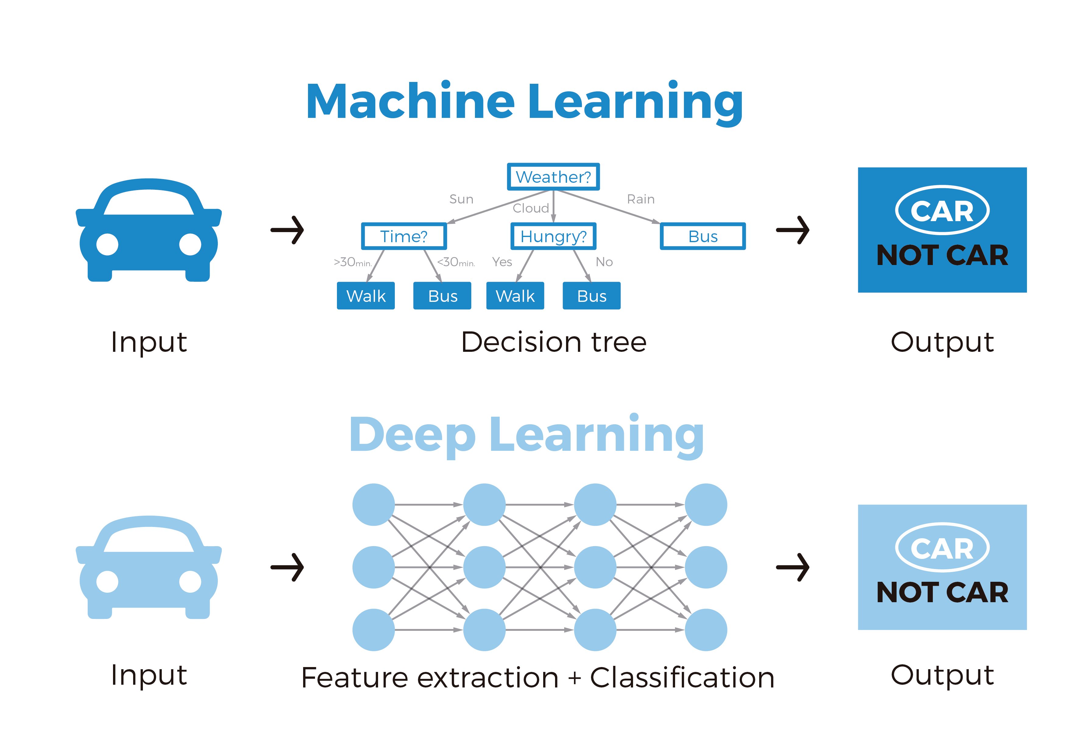
DL is a branch of ML that is implementing through large Artificial Neural Networks (ANN) of over 100 layers, and training such networks requires lots of labeled data and computational power. Its methods are based on learning data representations as opposed to task-specific algorithms, and learnings can be supervised, semi-supervised or unsupervised (and can be implemented in NLP or Reinforcement Learning).
(Source: blog.bismart.com, n.d.)
The need for DL comes when the volume of data increases, and ML techniques no matter how optimized becomes inefficient in terms of performance and accuracy. It is used in image classification, NLP, speech recognition and recommendation systems for example.
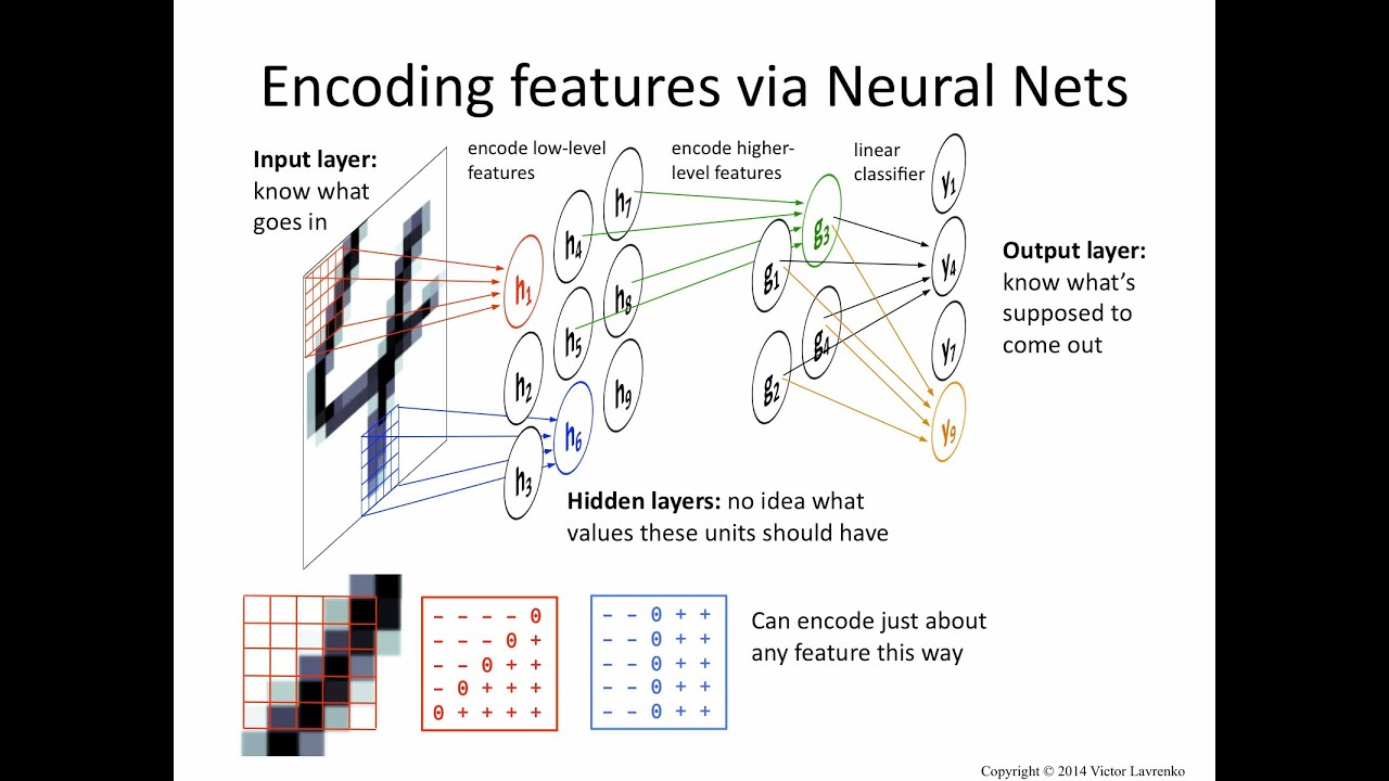
(Source: Victor Lavrenko, 2015 - Rough idea of encoding the features)
As described by Yann LeCun, Yoshua Bengio & Geoffrey Hinton, Deep Learning, Nature,
Deep learning allows computational models that are composed of multiple processing layers to learn representations of data with multiple levels of abstraction. It discovers intricate structure in large data sets by using the backpropagation algorithm to indicate how a machine should change its internal parameters that are used to compute the representation in each layer from the representation in the previous layer.
The distinct differences between ML is that DL is that in ML, features are provided manually whereas DL learns features directly from the data (remember the definition of a feature as an individual measurable property or characteristic of a phenomenon - e.g. age, sex, height etc.).

(Source: Facundo Bre et., 2017)
It starts with the Neural Network, which contains the Input layer - which takes in the -values and its features (e.g.
), the Hidden layers which contains Neurons with randomized weights for each features, and finally the Output layer, which classifies the value into the relevant prediction classes.
(Source: Shivlu Jain, 2017)
The artifical Neuron infers from the human brain cells (neuron) contained in the brain, that is surrounded by dendrites which receive signals from other neurons, and these signals are summed and forwarded to axons, and thereafter fired to the next neurons via the synapses if it exceeds a particular limit.
The Neural Network can be interpreted as the brain which contains the artifical Neurons.
(Source: SION, 2021)
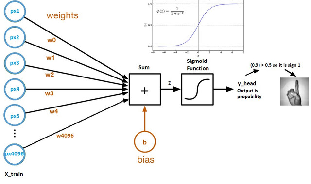
In each Neuron, just like it's biological counterpart, it receives an input, processes it and generates an output which is either sent to other Neurons for further processing or it becomes the final output.
Each input gets multiplied by a Weight, which is initialized randomly and updated during the model training process. After training, the network assigns higher Weight to the input it considers more important as compared to the ones which are less important.
As this process continues, the Neuron that are important gets "activated" and the non-important ones gets "deactivated" (which are simply percentages), sending "signal" to the next Neuron in the next layer (e.g. 0.0001 * 0.00002 will result in a lower "activation" value compared to 0.1 * 0.2 as the process goes on).
In addition to the Weights, another linear component is applied to the input called the Bias, to change the range of weight multiplied input. The Activation Function then takes in the sum of the Weights applied to previous computed output (or initial input) and the bias to return its current Neuron output.
This Bias is useful as say for example, setting bias greater than 10 would cause weights > 10 to be activated. Hence, the Bias tells how much the weighted sum needs to be meaningfully activated.
(Source: Omar Ghaffar, 2018)
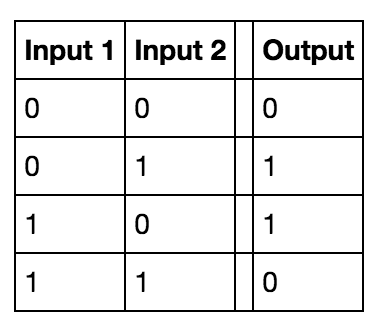
Another way to think of it is the XOR gate (explained in details here), where if all the inputs received in the Neuron is 0, the result is 0, and if there's any input that is 1, the result is 1 (maybe 0 depending on Weight and Bias calculations applied on inputs).


(Source: M. Kounelakis et., 2007) (Source: DeepAI.org, n.d.)
One of the most common example of ANN is the Multi-Layer Perceptron (MLP) - a class of the Feedforward NN, where each Neuron is connected to all Neurons in each layer(s).

(Source: Jacinta Chan et., 2016) (Source: Ajit Jaokar, 2019)
Recall the terminologies and concepts covered here, and remember the gradient descent algorithm.
The steps to making a Neural Networks starts with,
- Defining Network structure, such as the number of input, hidden and output layers, and neurons per layers.
- Initialise the model’s parameters, such as the weight and the biases randomly. Do not set large initial weight as it will lead to slower learning.
- For each epoch,
-
Implement Forward Propagation, the process which a Neural Network takes input data and keeps producing another value through all the subsequent layers, which implies that the network is "connected". For each Forward Propagation in each Neuron
and
prior outputs (or inputs),
Whereis the Activation Function,
the output for the previous computed output (or initial input),
the weight applied and
the bias.
-
Compute the loss using the output into a loss function. For example, using the Binary Cross-Entropy loss function (log-likelihood method for error estimate) for the Sigmoid Activation Function, where
is the number of training examples,
For the Softmax Activiation Function, the Categorial Cross-Entropy loss function is used as,
(Source: Raúl Gómez, 2018)
For ReLU and other Activation Functions, Mean Squared Error (MSE) loss function might be used instead.
-
Implement Backward Propagation, the process where the gradients - derivative of loss computed with regards to weights and parameters of the Neural Network are computed. It starts with computing the gradient of the parameters of the last layer, which computed gradient is used to compute the gradients of the prior layer and so on.
In summary, the information flows from right to left, compared to the Forward Propogation which starts from left to right.
As the gradients of the layer is found, the subsequent weight also gets updated by the gradient descent process (algorithms such as Adaptive Moment Estimation (AdaM) is usually preferred over the Stocashtic Gradient Descent (SGD), for more read here).
Note that SGD is different from Gradient Descent.
For each Backward Propagation, where
is the learning rate (slope of descent),
-
Remember that every Neurons contains the -weights (corresponding to the number of
features), and these weighted values gets passed on to the next layer Neurons (e.g.
), which the eventual output layer returns the number of final "features" depending on the number of neurons in the last hidden layer.
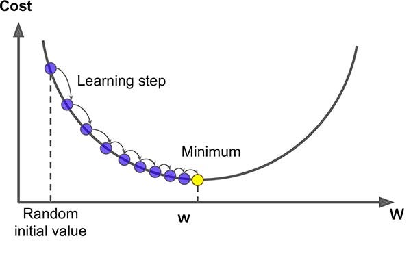

(Source: Agnes Sauer, 2020) (Source: @alkasm, 2017)
The gradient descent phase would reduce the derivative at each backpropagation which further gets in the chain of layers until convergence (reducing the weight size helps in reducing step size). Large step sizes can result in cost like < and > than prior cost value.
The final output of the -features prediction would be provided, and it's up to one to decide what to do with the values.
For example, one may take an average of the total prediction values and apply it using the Unit Step (or Binary Step) function to evaluate or classify if it belongs to a class in a boolean manner (0 or 1).
Sometimes due to imbalanced data, the threshold of the sigmoid function doesn't return 0.5, so another method is to (max + min) / 2. However, there are other better strategies to handle such scenarios.
Types of Activation Functions
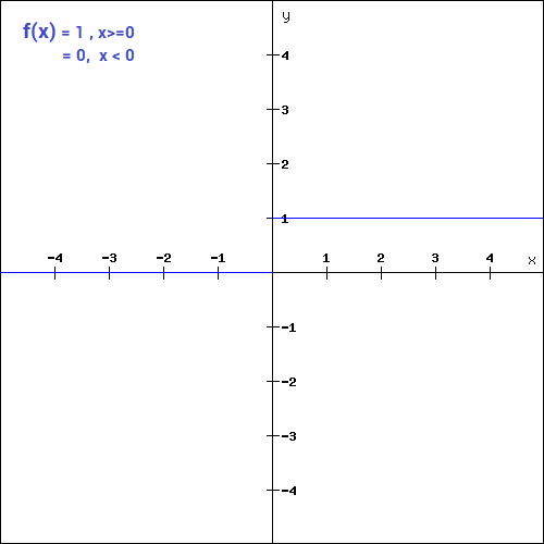

(Source: DISHASHREE GUPTA, 2020)
This could be used as a threshold based classifier if the neuron should be activated based on the value from the linear transformation.
This function is useful for creating a binary classifier.
The mathematical function is,
During the Backward Propagation, the weights and biases are not updated since the gradient of the function is 0 (which can be a hindrance in the Backward Propagation process because there are no adjustments and gradient descent won’t be able to make a progress in updating the weights).
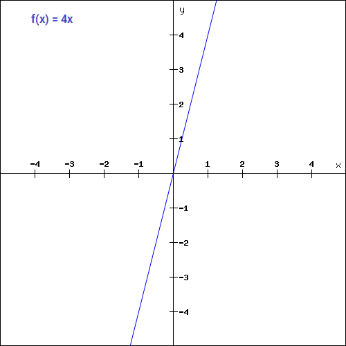

(Source: DISHASHREE GUPTA, 2020)
The mathematical function is (where is a constant value),
During the Backward Propagation process, the updating factor for all the weights and biases will be the same as the gradient is a constant which does not depend on the input value at all, hence the Neural Network will not really improve as the gradient is the same for every iteration and not be able to train well and capture complex patterns from the data.
This would be ideal for simple tasks where interpretability is desired.

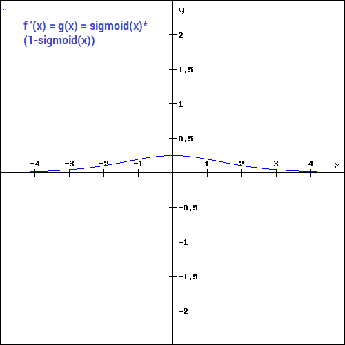
(Source: DISHASHREE GUPTA, 2020)
This is one of the most widely used non-linear function, and it transforms the values between the range 0 to 1.
The mathematical function is,
The gradient values as seen is significant for range -3 to 3 and gets flatter in other regions, which implies that values greater than 3 or less than -3, we will have very small gradients, hence as the gradient values approaches 0, the network isn't really learning.
The Softmax is a combination of multiple sigmoids, which each values return between 0 to 1, expressing probabiltiies of a data point belonging to a particular class (hence used for binary classification problems).
It is used for multiclass classification problems which returns the probability for a datapoint belonging to each individual class.
(Source: DISHASHREE GUPTA, 2020)
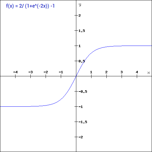
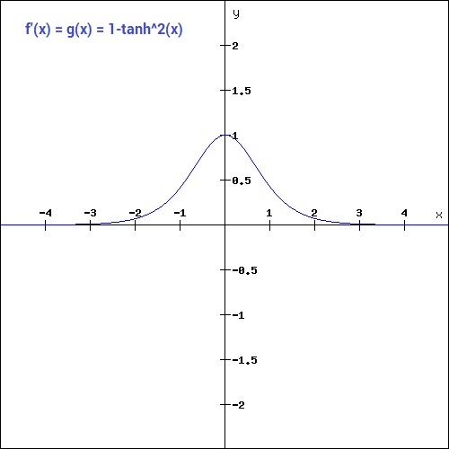
The tanh function is similar to the sigmoid function except that it is symmetric around the origin, with range of values from -1 to 1.
The mathematical function is,
The gradient of the tanh function is steeper compared to the sigmoid function. Since it is centered around 0 (symmetrical from -1 to 1), it is preferred as it does not restrict the gradients to move in a certain direction (e.g. only positive).
(Source: DISHASHREE GUPTA, 2020)
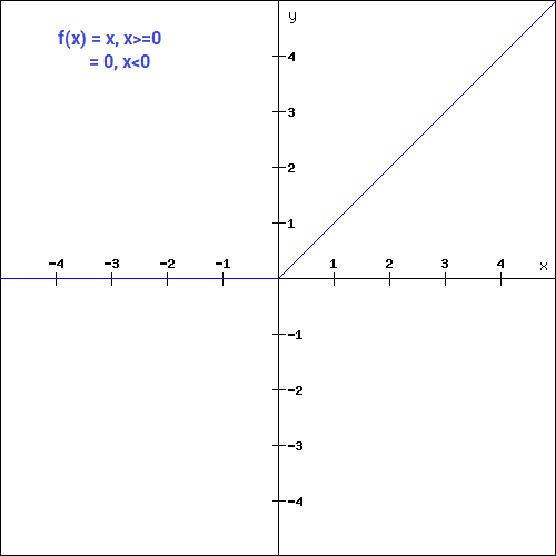
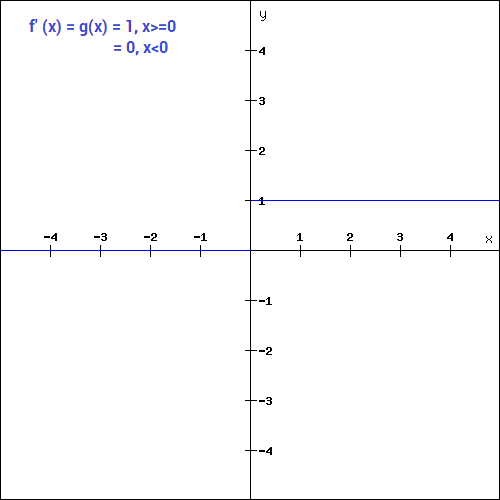
The Rectified Linear Unit (ReLU) function, unlike other Activation Functions, does not activate all Neurons at the same time, as the Neurons will only be deactivated if the output of the linear transformation is less than 0.
Since only a certain number of Neurons are activated, it makes the computation more efficient compared to the rest of the Activation Functions.
During the Backward Propagation process, the weights and biases for some Neurons will not be updated.
The mathematical function is,
(Source: DISHASHREE GUPTA, 2020)
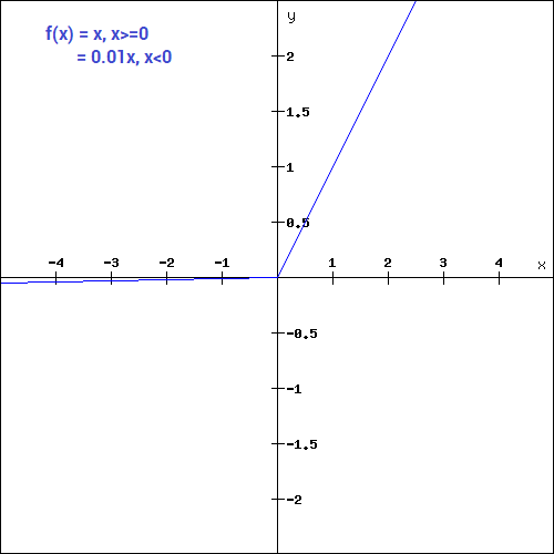
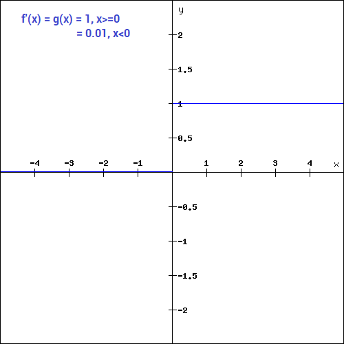
The mathematical function is,
Instead of defining 0 for negative values, it produces an extremely small linear component, which would no longer produce dead Neurons in that region (except less active).

(Source: DISHASHREE GUPTA, 2020)
The mathematical function is,
The "constant" value is a "trainable" parameter that can be learnt for faster and more optimum convergence.
(Source: DISHASHREE GUPTA, 2020)
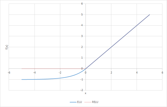
The mathematical function is,
Compared to the Parametric and Leaky ReLU, instead of a straight line, it uses a log curve for defining the negative values, and is shown to obtain higher classification accuracy than ReLU.
(Source: Lilian Weng, 2017)
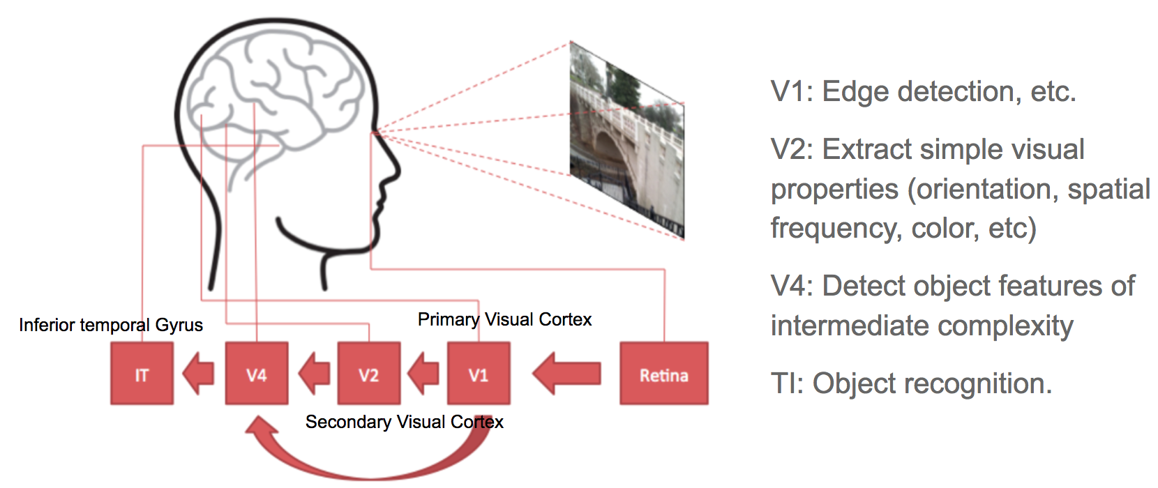
CNN is a type of Feed-Forward ANN, which connectivity pattern between its neurons is inpsired by the organization of the visual cortex system.
The primary visual cortex (V1) does edge detection out of the raw visual input from the retina.
The secondary visual cortex (V2) receives the edge features from V1 and extracts simple visual properties such as orientation, spatial frequency and color.
The visual area (V4), like V2 handles orientation, spatial frequency and color, but is tuned for object features of intermediate complexity such as simple geometric shapes. It also receives direct input from V1.
The Inferior temporal Gyrus (IT) then processes and recognizes the information of "what" something is (such as faces).


(Source: PULKIT SHARMA, 2018)
For example, like the V1, we want to detect the edges from the images. To do so, we take only 1-channel image (6 × 6), where grayscale pixels range from 0 (black) - 255 (white).


(Source: PULKIT SHARMA, 2018)
Next, we convolve this (6 × 6) matrix with a (3 × 3) filter (also known as the kernel), which would result in a (4 × 4) image. For example in above, we show only 2 steps of the process where each segment of the matrix is multiplied with the filter (blue matrices). Doing so for all the segments of the matrix should result in the above (last matrix).
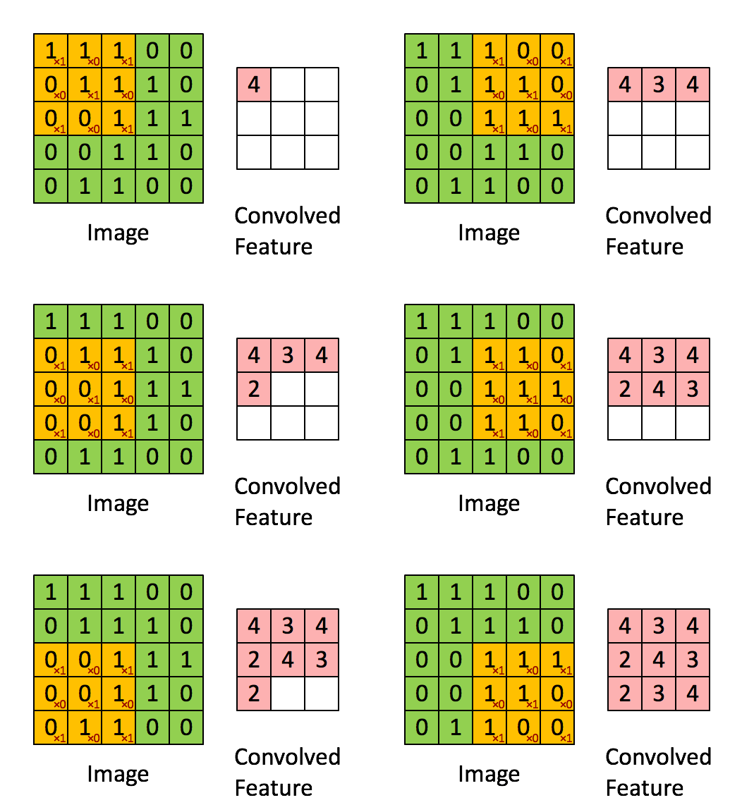
(Source: Sumit Saha, 2018 - Animated idea of the convolution operation)

(Source: PULKIT SHARMA, 2018)
To understand how the above filter works, the higher pixel values represents the brighter portion of the image and the lower pixel values represents the darker portions. Using this derivation gives us the vertical edge in an image.


(Source: PULKIT SHARMA, 2018)
These are examples of several other filters that can be used to detect edges.

(Source: Ayeshmantha Perera, 2018)
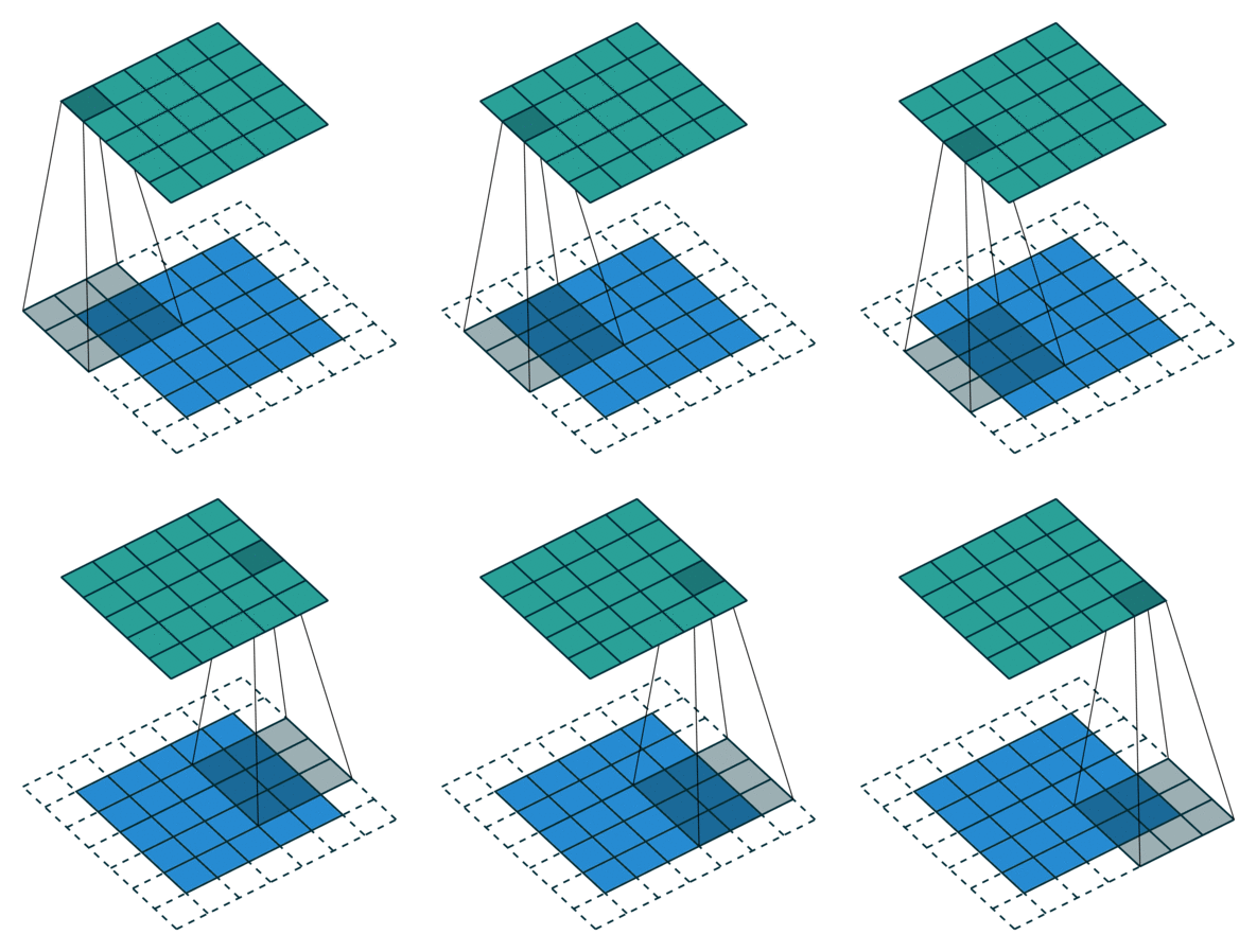
(Source: Sumit Saha, 2018)
From the above examples, we see that after the convolutional operation, the size of the image matrix shrinks, and the pixels present in the corner of the image are used only a few number of times during the operation as compared to the central pixels, which leads to information loss.
The solution is to append paddings (aka additional borders), such as adding 1-pixel all around the edges, making a (8 × 8) matrix which would result in the original (6 × 6) matrix size after the operation.
| Input | Padding | Filter size | Output |
|---|---|---|---|
n × n
|
p |
f × f
|
(n + 2p - f + 1) × (n + 2p - f + 1)
|
The common choice for padding p size can be p = (f - 1) / 2. Using padding is known as Same padding and no padding is Valid padding.

(Source: Shyam Krishna Khadka, 2017)
Another form of convolution is the strided convolution, we take s + 1 steps instead of 1, both in the horizontal and vertical directions separately, leading into,
| Input | Padding | Stride Step | Filter size | Output |
|---|---|---|---|---|
n × n
|
p |
s |
f × f
|
[(n + 2p - f) / (s + 1)] × [(n + 2p - f) / (s + 1)]
|

(Source: PULKIT SHARMA, 2018) (Source: Sumit Saha, 2018)
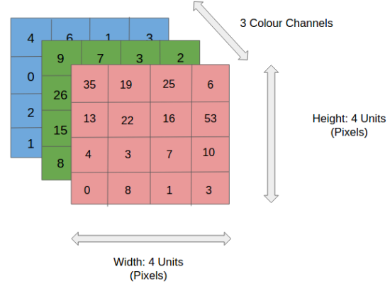
For scenarios where instead of a 2D-input image, we have a 3D-input image, we use a (n × n × d) filter.
For example of a (6 × 6 × 3) image, we use a (3 × 3 × 3) filter instead.
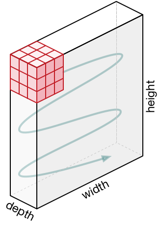
(Source: Sumit Saha, 2018)
Since there are 3 channels in the input, the filter will also have 3 channels, and it should result in a (4 × 4) matrix.
The first element output is the sum of the element-wise product of the first 27 values from the input (9 values from each channel) and 27 values from the filter. The subsequent operations is then done to the rest of the matrix.
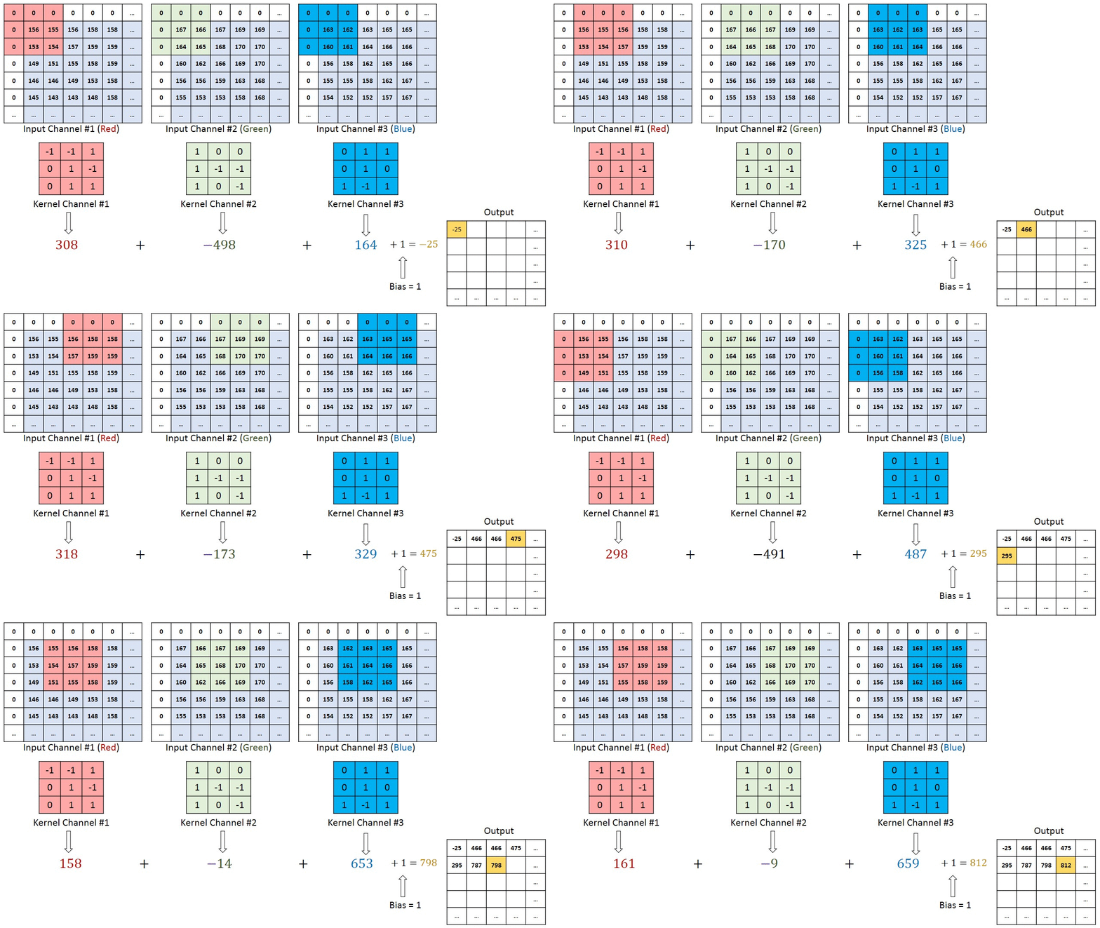
(Source: Sumit Saha, 2018 - Animated idea of the convolution 3D operation)
It can be represented as (where nc is the number of channels and nf the number of filters),
| Input | Padding | Stride Step | Filter size | Output |
|---|---|---|---|---|
n × n × nc
|
p |
s |
f × f × nc
|
[(n + 2p - f) / (s + 1)] × [(n + 2p - f) / (s + 1)] × nf
|
These can be eventually formatted as a layer in the ANN where,
Using the above example of (6 × 6 × 3) input , the (
3 × 3 × 3) filters are the weights . These activations from layer 1 act as the input for layer 2 and so on.
The number of parameters in the case of CNN is independent of the size of the image size, as it depends on the filter size instead.
Since we have 3 (3 × 3) filters, and there is a bias term for each filter, the total number of parameters is 3(3 * 3) + 3 = 30.
The following is the hyperparameters for the layer,
-
f: The filter size. -
p: The padding size. -
s: The stride step size. -
nf: The number of filters.
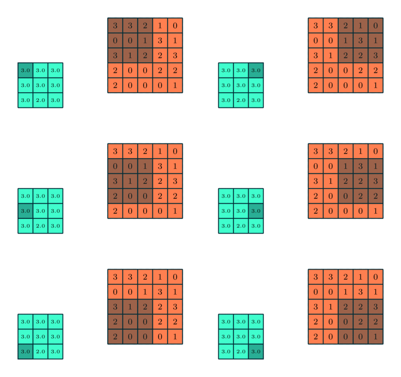
(Source: Sumit Saha, 2018 - Animation of pooling)
Pooling layers are generally used to reduce the size of the inputs and hence speed up the computation.


(Source: PULKIT SHARMA, 2018)
For the example above, for each consecutive (2 × 2) block, we take the max number (this is known as max pooling), and applied a filter of size 2 and stride size 2.
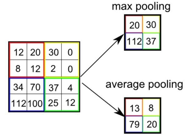
(Source: Sumit Saha, 2018)
There are 2 types of pooling,
- Max Pooling: Returns the maximum value from the portion of the image covered by the kernel.
- Average Pooling: Returns the average of all the values from the portion of the image covered by the kernel.
Max pooling is generally preferred as it performs as a noise suppresent, since it discards the noisy activations altogether and performs de-noising along with dimensionality reduction.
The following is the hyperparameters for the layer,
-
f: The filter size. -
s: The stride step size. - Using max or average pooling.
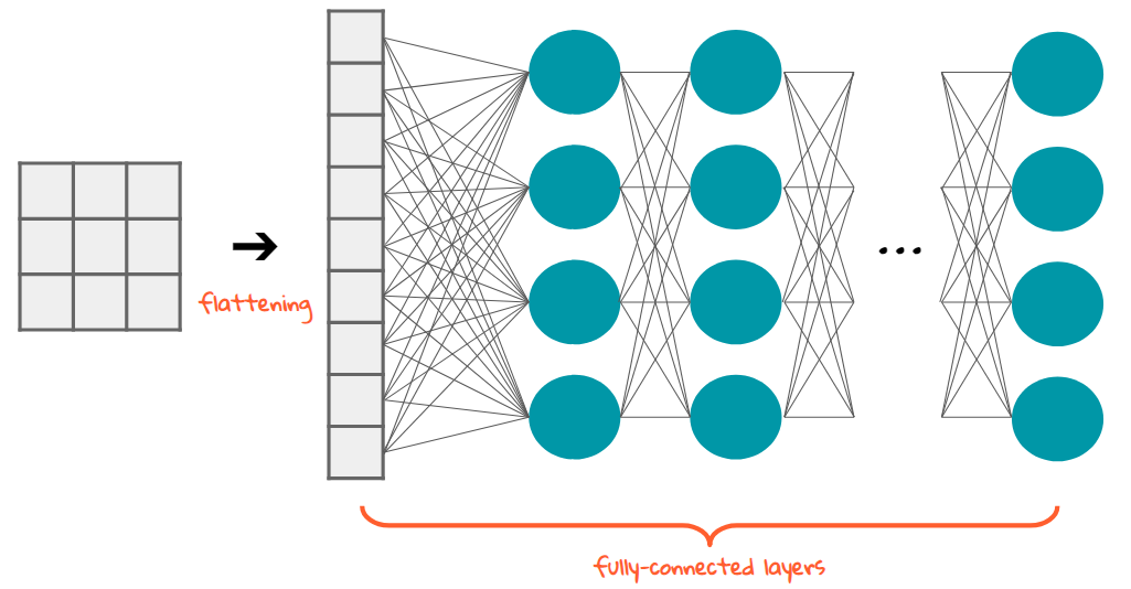
(Source: Jiwon Jeong, 2019)
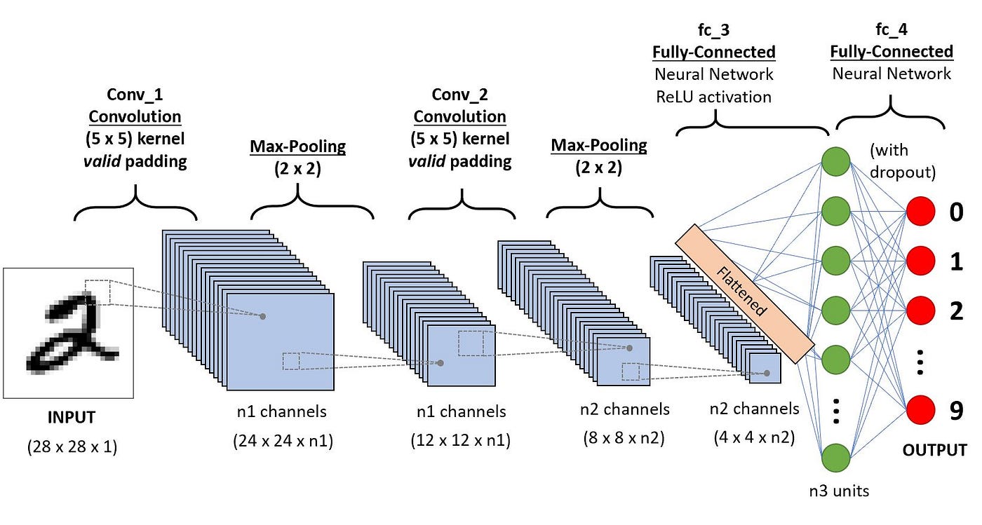
Before the data gets classified, the data needs to be converted into a 1-dimensional array to input to the next layer. It flattens the output of the convolutional layer to create a single long feature vector, and is connected to the final classification model (fully connected layer). Think of it as putting all the pixel data into one line to make connections with the final layer.
(Source: Sumit Saha, 2018)
Putting it all together, the fully connected layer is the Neural network that translates into the category of classification (e.g. cat or dog?).
These are the common types of networks,

(Source: PULKIT SHARMA, 2018)
This takes a grayscale image as an input, and passes through a combination of convolution and pooling layers, which output will be passed through the fully connected layers and classified into the corresponding classes.
-
Parameters:
60k - Activation function: Tanh
The example flow is,
1. Convolution
2. Pooling
3. Convolution
4. Pooling
5. Fully connected (L1)
6. Fully connected (L2)
7. Output

(Source: PULKIT SHARMA, 2018)
Similar to LeNet except with more convolution and pooling layers.
-
Parameters:
60million - Activation function: ReLu

(Source: PULKIT SHARMA, 2018)
The underlying idea behind was to use a much simpler network by having convolution layers that have (3 × 3) filters with a stride of 1. The max pool layer is used after each convolution layer with a filter size of 2 and a stride of 2.
-
Parameters:
138million - Activation function: ReLu
(Source: Connor Shorten, 2019)

(Source: @thebrownviking20, 2018)
There are problems like vanishing gradient problem, where some gradients through the process of repeated multiplication gets reduced and completely vanish, resulting in decay of information over time, as no learning is taking place with no gradients. To resolve this, whilst training deep networks, we can use Residual blocks to help in the training to reduce such problems.
For example, this the general flow of calculating activations,


(Source: PULKIT SHARMA, 2018)
To add residuals, we derive to,


(Source: PULKIT SHARMA, 2018)
Which results in this equation,

(Source: PULKIT SHARMA, 2018)
The benefits of using such is that the training error does not increase as more layers are added (causing information loss).
(Source: Lilian Weng, 2017)
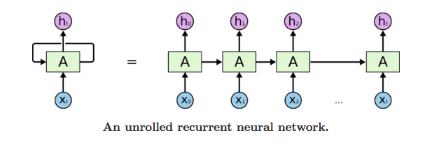
The model's chain-like nature intuitively relates to sequences and lists. It processes one element in the sequence at one time step, which result is passed to the next to facilitate the compution of the next element.
In short, it uses their internal state (memory) to process sequences of inputs, which enables it to process long sequential data to tackle tasks with context spreading in time.
One example is reading a Wikipedia article, where the model reads character by character and predicts the following words given the context.

(Source: BAI3, 2021)
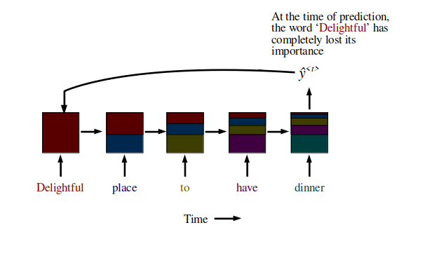
Another example of its use-case is in NLP, where each sentence can have a variable number of tokens. For example, the sentence "Delightful place to have dinner" results in 5 token, but "Food was nice but service wasn’t’" is 6, resulting in a mismatch. Even using the maximum sentence token length may also create astronomically high number of parameters making it least performant.
Here's a basic idea of a RNN cell,

(Source: Fisseha Berhane, n.d.)
In RNN, you have multiple repetitions of the same cell. For example, a sentence "Delightful place to have dinner" becomes x1 = "Delightful", x2 = "place", x3 = "to", x4 = "have", x5 = "dinner" (means 4 time steps).
Below is an example,

(Source: BAI3, 2021)
(Source: Lilian Weng, 2018)
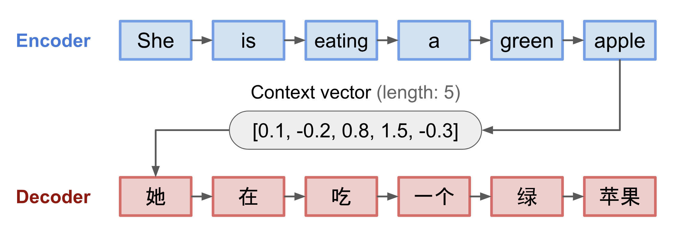
One familar example can be used is translation, that is done using the Encoder and Decoder model (e.g. Seq2seq), which contains 2 parts,
- Encoder that processes input sequence and compresses the information into a context vector (aka sentence embedding/"thought" vector) of a fixed length. It is expected to be a good summary of the meaning of the whole source sequence.
- Decoder that emits the transformed output.
(One disadvantage is that it requires a fixed length)
However, RNN suffers from short-term memory. If the sequence is long enough, there might be a problem carrying information from earlier time steps to later ones and it may leave out important information from the beginning - this is a result of vanishing gradient as mentioned earlier.
(Source: BAI3, 2021)
The solution to tackle these vanishing gradient problem is to use LSTM and GRU RNN units.

(Source: Fisseha Berhane, n.d.)
This contains the following components,
-
Forget gate: Keeps track of the memory to forget. For example in a sentence, if the subject changes from a singular word to a plural word, get rid of the previously stored memory value.
-
Update gate: Updates to reflect the latest state. For example in a sentence, if the new subject is plural, update the subject to become plural.
-
Output gate: Decides what the output should be given out.
The previously factored importance would get reflected into the next subsequent time states.
(Source: Liqing Wei et., 2020)
This contains the following components,
-
Update gate: Similar to the forget gate of an LSTM. It decides what information to throw away and add.
-
Reset gate: Decides how much past information to forget.
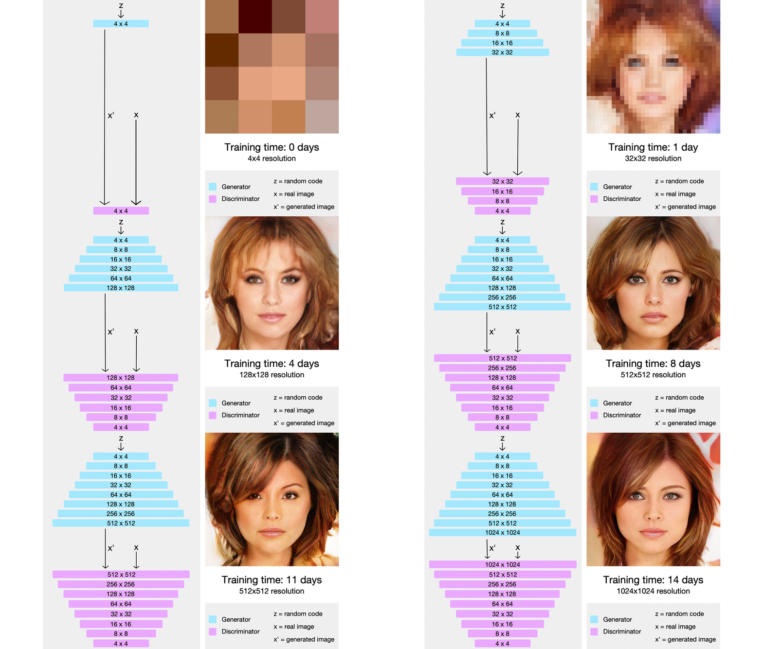
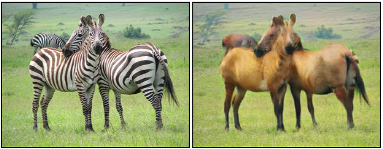
(Source: Ajay Uppili Arasanipalai, 2019 - 1st being the process of each epoch generating a new fake data, and 2nd a result of such)
The idea is to use two neural networks, pitting one against the other (thus the "adversarial"), in order to generate new, synthetic instances of data that can pass for real data. They are used widely in image generation, video generation and voice generation.
These are the few ways GAN can be used too, such as translating text into images or faces into emoji,
(Source: HARSH_DHAMECHA, 2021)
It is made up of 2 components, the Generator that generates new data instances, and the Discriminator that tries to distinguish the generated/fake data from the real dataset.
(Source: HARSH_DHAMECHA, 2021)
The Discriminator algorithm tries to classify the input data, and predict the label or category the data belongs. They are concerned soley with the correlation. The Generator algorithm does the opposite, it simply attempts to predict features based on a given label.
The Generator network is fed noise (e.g. random distribution) generates fake data from the noise before it is inputted to the Discrimator.
-
Phase 1: Generator is fed random data, and creates some random images given to the Discriminator, which then takes classifies these fake noises using the random images and actual iamges. The difference between the predicted and actual results are backpropagated through the network and the weights of the Disciminator is updated (note that the Generator is not trained or updated in this phase).
-
Phase 2: The produced fake images are then given to the Discrimator again and this time, real images are not given for comparison. The Generator learns by tricking the Discriminator into outputting false positives, and the Discriminator outputs probabilities which are assessed against the actual results and the weights updated from the prior backpropagation (note that the Discrimanator is not trained or updated in this phase).
(Source: Seiichi Uchida et., 2019)
However, in some cases, the Generator produces only a single sample, and learns to trick the Discriminator with a single image or a few images to believe as real image.
Another involves the generator and discriminator oscillating during training, rather than converging to a fixed point. If one agent becomes much more powerful than the other, the learning signal to the other agent becomes useless, and the system does not learn.
One of the methods to improve such is to use Deep Convolution GAN.

(Source: Deepak Birla, 2019)

(Source: Francois Chollet, 2016)
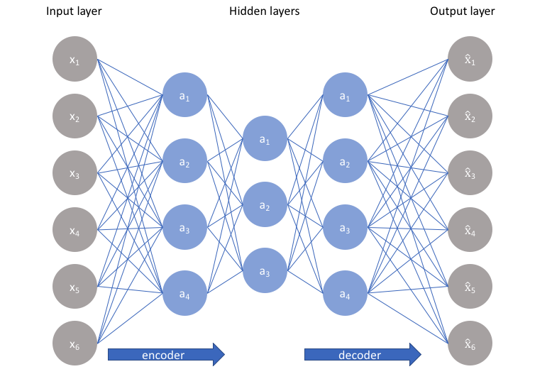
(Source: JEREMY JORDAN, 2018 - ANN view)
Auto-encoding is a data compression algorithm.
They are data-specific, meaning they will only be able to compress data similar to what they have been trained on.
They are also lossy, which means that the decompressed outputs will be degraded compared to the original inputs (similar to MP3 or JPEG compression) as opposed to lossless compression.
They are learned automatically from data examples, and doesn't require any new engineering but just appropriate training data.
It consists of the Encoder that maps the input into the Code (see bottleneck), and the Decoder that maps the Code to a reconstruction of the input.
The practical applications of autoencoders are data denoising and dimensionality reduction for data visualization.
In Q-learning, the formula is represented as such,

(Source: rubikscode.net, 2019)
With the Q-table matrix and model represented as such,


(Source: rubikscode.net, 2019)
In the case of Deep Q-Learning (DQL), it utilises ANN by creating the Q-Network that makes the action decision.

(Source: Philip Ossenkopp, 2018)

(Source: rubikscode.net, 2019)
