Part 4: Clustering - oooookk7/machine-learning-a-to-z GitHub Wiki

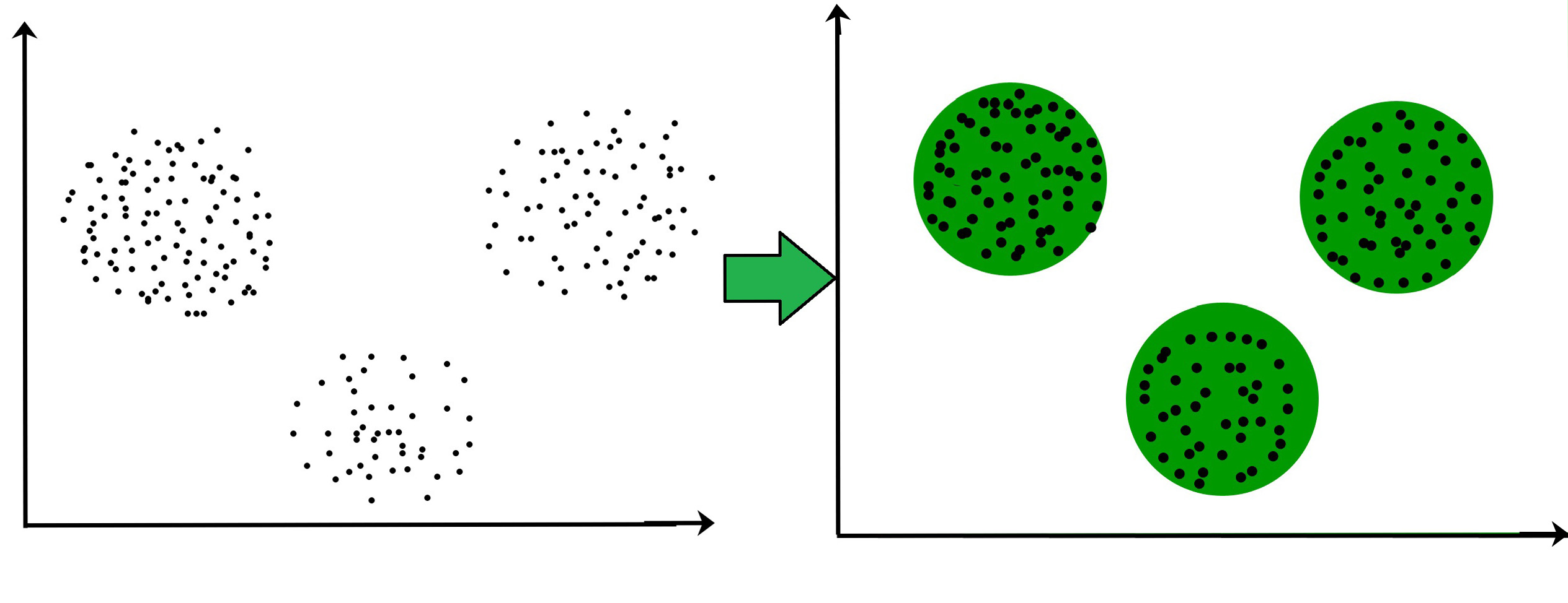
(Source: Surya Priy, 2020)

Clustering is the task of dividing the data points into a number of groups (or classes) that have (more) similarities to each other. It is often used as a data analysis technique for discovering patterns or groups in the present unlabeled data set. The criteria for a good clustering depends on the use-case or requirements (e.g. finding "natural clusters" for unknown properties or suitable groupings or outlier detection).

(Source: Ahmed M. Fahim, 2018 - Example of density-based methods)

(Source: Jeong-Hun Kim et., 2019 - Another example of density-based methods)

(Source: Abhijit Annaldas, 2017 - Breakdown of a point in density-based methods)

(Source: RAINERGEWALT, 2020 - Example of hierarchical-based methods)

(Source: Amit Saxena et., 2017 - Example of partitioning methods)

(Source: Arvind Sharma et., 2016 - Example of grid-based methods)

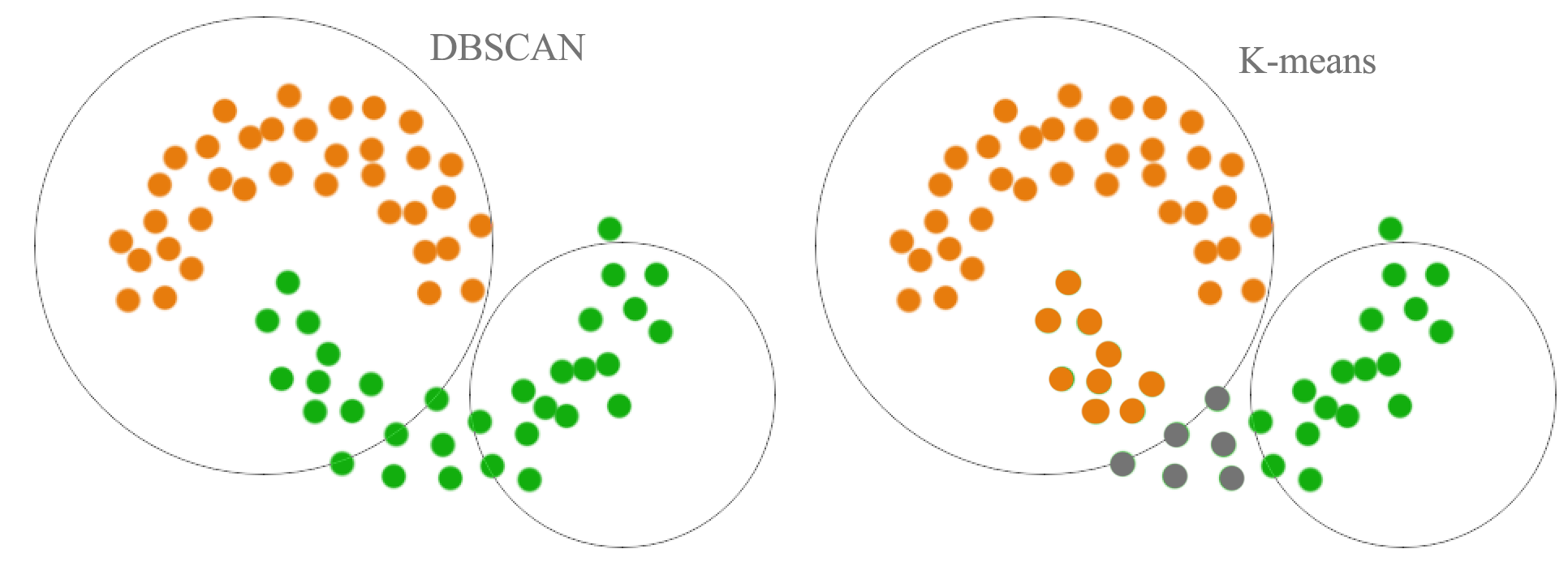
(Source: Jonathan Hui, 2017 - Comparison of k-means vs DBSCAN)

• Density-Based methods: These consider dense regions having some similarity (as clusters) and not the lower dense region of the space.

  • Terminologies are the core (starting point), border (the circled area surrounding with the radius of epsilon) and outlier which is a noise point that cannot be reached from the neighbouring points (and its subsequent neighbouring points).
  • It starts with the core point, which reaches the neighbouring points that are within the epsilon border (margin), which neighbouring points do the same to reach its neighbouring points until there are no more points it can reach. Points that are unreachable are called outlier points.
  • It is able to merge 2 clusters and tend to be more accurate.
  • Examples include Density-based spatial clustering of applications with noise (DBSCAN) and Ordering points to identify the clustering structure (OPTICS).

• Hierarchical-Based methods: These forms a tree-type structure based on hierarchy.

  • Types of this method are:
    • Agglomerative: Bottom-up approach where algorithm starts data points as individual single clusters until it becomes a singular large cluster.
    • Divisive: Top-down approach and the reverse of the bottom-up approach.
  • Examples include CURE (Clustering Using Representatives) and BIRCH (Balanced Iterative Reducing Clustering and using Hierarchies).

• Partitioning methods: Partitions the data set into k-clusters and each partition forms a cluster.

  • This is used to optimize objective criterion similarity function (e.g. distance as parameter).
  • Examples include k-means and CLARANS (Clustering Large Applications based upon Randomized Search).

• Grid-based Methods: Data space is formulated into a finite number of cells to form a grid-like structure, and clustering operations are done on these grids ar fast and independent of the number of data points.

  • Examples include STING (Statistical Information Grid) and CLIQUE (CLustering In Quest) (for its implementation in python read here).

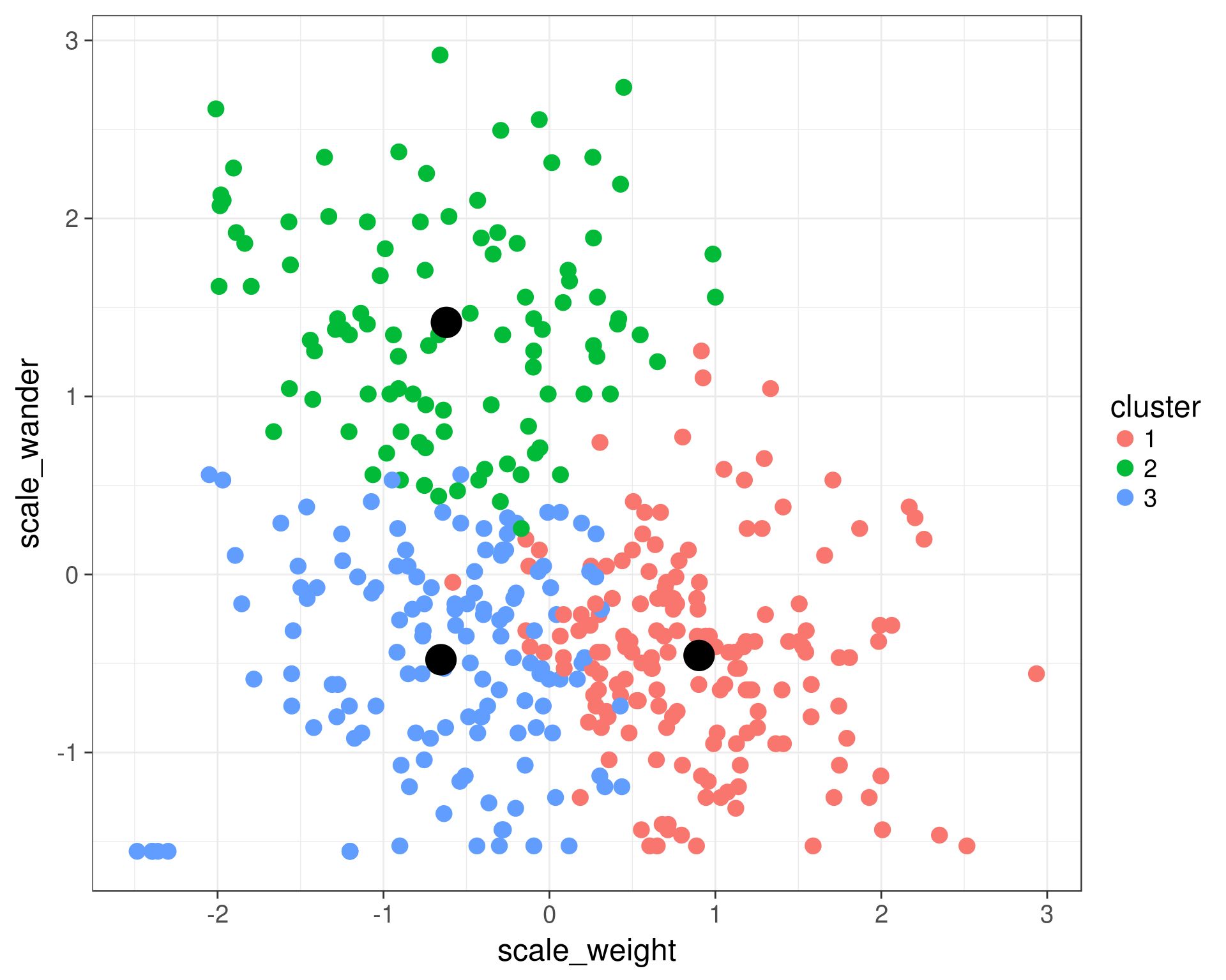
(Source: Ann Arbor R User Group, n.d.)

k-means is a centroid-based or distance-based algorithm that calculates distances to assign a data point to a cluster, where each cluster is associated with a centroid data point. Its main objective is to minimize the sum of the distance between the points and their respective cluster centroid and maximize the difference between clusters.

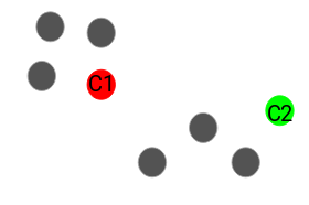
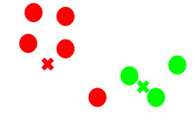
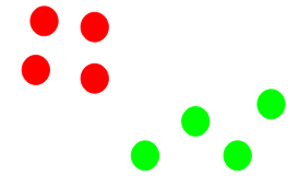
(Source: Pulkit Sharma, 2019 - Visual description of k-means clustering)

It can be formally described as this (uses Eucleadian distance to calculuate distance),

Where represents the set of all clusters, the data point and the mean (or centroid data point) for cluster .

In summary, the algorithm works like this,

1. Random choose data points to become the centroid of the cluster.
2. Starting from the first data point, compare the distances between the various clusters centroid data points. The cluster with the smallest distance becomes the assigned cluster.
3. Repeat step 2 until all data points are assigned.
4. Repeat step 1 and 3 for several iterations and choose the assigned clusters with the least variance within each cluster.

As the number of clusters we choose for a given dataset is not random, we would need to find out the right number of clusters that we should choose. Since each cluster is formed by calculating and comparing the distances of data points within its cluster centroid, we can use the Within-Cluster-Sum-of-Squares (WCSS) to find the right number of clusters.

Where is the set of all clusters, and the centroid data point of the cluster .

The idea is to minimize the sum and to find the right threshold value, the Elbow point graph can be used to find the optimum value for , by randomly initialising the k-means algorithm for a range of values which we will plot it against the WCSS for each value.

Generally, the optimum value for is 5, as the drop is minimal starting from 5 for the WCSS.

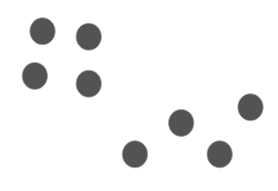
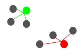
(Source: Pulkit Sharma, 2019 - Visual description of k-means++ selection)

As an extension of the original k-means algorithm, it does not choose the centroid randomly but rather uniformly,

1. Choose the first cluster centroid at random from the data points that we want to cluster.
2. Compute the distance of each data point from first cluster center.
3. Choose the new cluster centroid from the data points that has the probability of being proportional to the distance .
4. Repeat steps 2 and 3 until all clusters have been choosen.

(Source: Pulkit Sharma, 2019)

Hierarchical clustering algorithm groups similar objects into clusters, where it builds a hierarchy of clusters, and each cluster is distinct from each other and data points within each cluster are broadly similar to each other.

(Source: Pulkit Sharma, 2019)

Considered as the bottom-up approach, by assigning each point to an individual cluster in this technique. Suppose there are 4 data points, then each data points are assigned to individual clusters. Then at each iteration, the closest pair of clusters are merged, and this step is repeated until a single cluster is left.

This process of merging (or adding) clusters at each step is known as additive hierarchical clustering.

(Source: Pulkit Sharma, 2019)

Considered as the bottom-up approach, it works in the opposite way of the agglomerative approach. It starts with a single cluster and assigns all points to the cluster. At each iteration, we split the farthest point in the cluster and repeat this process until each cluster contains a single data point.

In this description, we will be using the agglomerative approach (and single link merging). For an example of a data set with 5 data points,

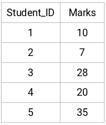
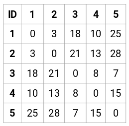
(Source: Pulkit Sharma, 2019 - Step 1 of creating the proximity matrix)

(Source: Pulkit Sharma, 2019 - Step 2 assign each data point to an individual cluster)

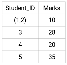
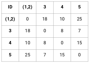
(Source: Pulkit Sharma, 2019 - Step 3 of merging individual clusters from the proximity matrix)

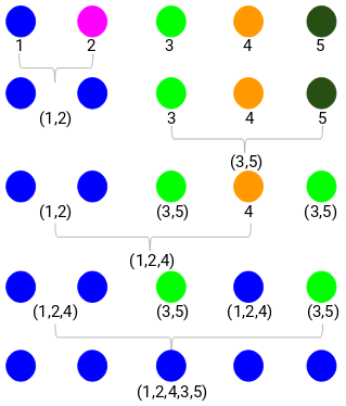
(Source: Pulkit Sharma, 2019 - Step 4 progressing of merging clusters into a single cluster)

For Euclidean distance,

In summary,

1. Create the proximity matrix for data set for all data points in the data set . This can be calculated using the Euclidean distance (or Manhattan distance), where for 2 data points for features.
2. Assign every data points to an individual cluster.
3. Find the smallest distance in the proximity matrix and merge the data points. Then update the proximity matrix.
4. Repeat step 3 until only a single cluster is left.

From step 4, we can construct a dendrogram to find the optimal number of clusters to choose,

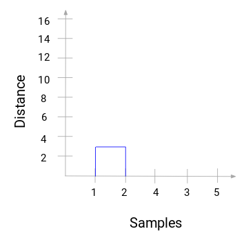
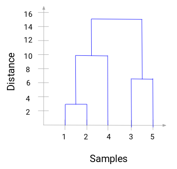
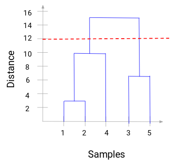
From this, we can visualize the steps of the hierarchical clustering clearly, where the more the distance of the vertical lines in the dendrogram, the wider the distance between the clusters.

Choosing the number of clusters will be the number of vertical lines intersected by the line drawing using the threshold. In the example, since the red dotted line intersects 2 vertical lines, we will use 2 clusters instead.

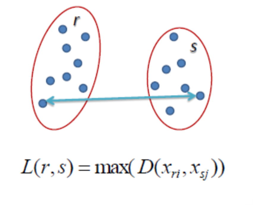
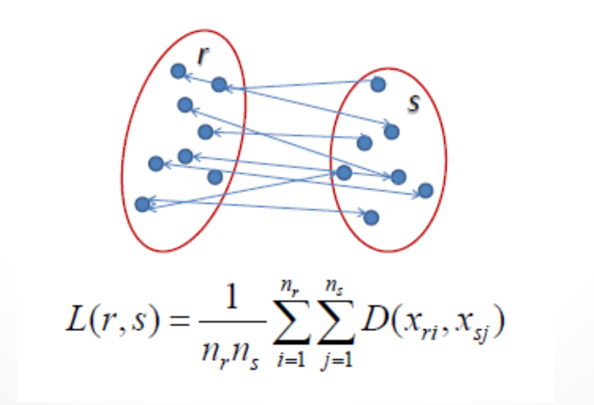
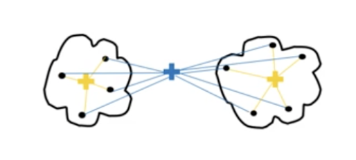
(Source: Cory Maklin, 2019 - From left to right, Single linkage, Complete linkage, Average linkage, and Ward linkage)

The linkage criteria refer to how the distance between clusters is calculated during its merging process.

• Single linkage: Find the minimum between each data point to make them into a cluster where
  
  
  

• Complete linkage: Find the maximum between each data point to make them into a cluster where
  
  
  

• Average linkage: Find the average for all data point in each cluster to make them into a cluster where
  
  
  

• Ward linkage: Find the sum of squared differences for all data point in each cluster to make them into a cluster. Starts with the merged cluster sum squared differences (new mean derived from merge) subtracting the subsequent clusters sum squared differences.
  
  
  

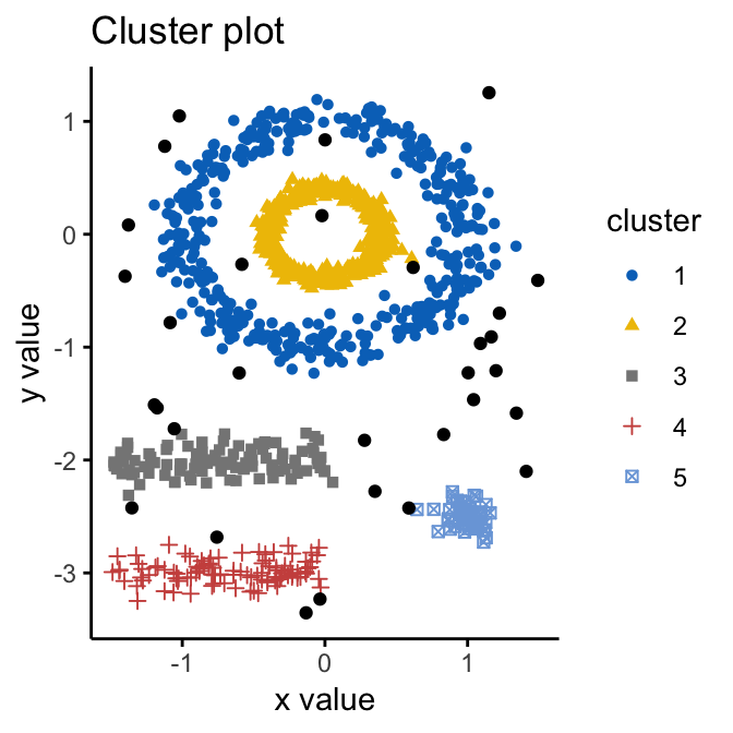
(Source: Alboukadel Kassambara, n.d.)

Density-based spatial clustering of applications with noise (DBScan) is a density-based clustering algorithm that seeks areas in the data that have a high density of observations versus areas of data that are not very dense with observations. It is able to sort data into clusters of varying shapes well, is robust to outliers, and does not require the number of clusters to be specified beforehand.

There are 2 parameters required,

• Epsilon: The radius of the neighbouring circle to be created around each data point to check for density.
• Min Points: The minimum number of data points required inside the neighbouring circle to be classified as a core point.

(Source: Evan Lutins, 2017)

It starts with every data point and creates a neighbouring circle of epsilon radius around it. These points are then classified into:

• Core point (>= min points): The data point is classified as such if it contains at least the number of min points in its neighbouring circle (note that distance is calculated generally using Euclidean distance).
• Border point (< min points and > 0): If it has data points in its neighbouring circle but less than the required number of min points in its neighbouring circle.
• Noise point (= 0): If there are no data points in its neighbouring circle.

Reachability is when a data point can be accessed from another data point directly or indirectly. Connectivity is when 2 data points belong to the same cluster or not.

(Source: Abhishek Sharma, 2020)

Point X is directly density-reachable from point Y if Y is a core point and if X belongs to and is within the neighbourhood of Y. In the example above, X is directly density-reachable from Y, but it is not true for the inverse.

(Source: Abhishek Sharma, 2020)

Point X is density-reachable from point Y if there is a chain of points Y > P1 > ... > Pn > X such that it is directly density-reachable from a core point in the chain (e.g. P2 > X). In the example above, X is density-reachable from Y from Y > P3 > P2 > X, but it is not true for the inverse.

(Source: Abhishek Sharma, 2020)

Point X is density-connected from point Y if there exists a point O such that both X and Y are density-reachable from O. In the example above, both X and Y are density-reachable from O (from core points A, B, O) hence we can say X is density-connected from Y.

(Source: Abhishek Sharma, 2020)

Clusters are formed when data points are density-connected to each other. Notice that noise points are ignored and aren't part of the cluster.