Statistics for Software - oleksiyp/oleksiyp.github.io GitHub Wiki

Non-parametric statistics gave us quantiles, but offers so much more. Generally, non-parametric describes any statistical construct that does not make assumptions about probability distribution, e.g. normal or binomial. This means it has the most broadly-applicable tools in the descriptive statistics toolbox. This includes everything from the familiar histogram to the sleeker kernel density estimation (KDE). There’s also a wide variety of nonparametric testsaimed at quantitatively discovering your data’s distribution and expanding into the wide world of parametric methods.

Parametric statistics contrast with non-parametric statistics in that the data is presumed to follow a given probability distribution. If you’ve established or assumed that your data can be modeled as one of the many published distributions, you’ve given yourself a powerful set of abstractions with which to reason about your system. We could do a whole article on the probability distributions we expect from different parts of our Python backend services (hint: expect a lot of fish and phones). Teasing apart the curves inherent in your system is quite a feat, but we never drift too far from the real observations. As with any extensive modeling exercise, heed the cautionary song of the black swan.

Inferential statistics contrast with descriptive statistics in that the goal is to develop models and predict future performance. Applying predictive modeling, like regression and distribution fitting, can help you assess whether you are collecting sufficient data, or if you’re missing some metrics. If you can establish a reliable model for your service and hook it into monitoring and alerting, you’ll have reached SRE nirvana. In the meantime, many teams make do with simply overlaying charts with the last week. This is often quite effective, diminishing the need for mathematical inference, but does require constant manual interpretation, doesn’t compose well for longer-term trend analysis, and really doesn’t work when the previous week isn’t representative (i.e., had an outage or a spike).

Categorical statistics contrast with numerical statistics in that the data is not mathematically measurable. Categorical data can be big, such as IPs and phone numbers, or small, like user languages. Our key non-numerical metrics are around counts, or cardinality, of categorical data. Some components have used HyperLogLog andCount-Min sketches for distributable streaming cardinality estimates. While reservoir sampling is much simpler, and can be used for categorical data as well, HLL and CMS offer increased space efficiency, and more importantly: proven error bounds. After grasping reservoir sampling, but before delving into advanced cardinaltiy structures, you may want to have a look at boltons ThresholdCounter, the heavy hitters counter used extensively in PayPal’s Python services. Regardless, be sure to take a look at this ontology of basic statistical data types.

Multivariate statistics allow you to analyze multiple output variables at a time. It’s easy to go overboard with multiple dimensions, as there’s always an extra dimension if you look for it. Nevertheless, a simple, practical exploration of correlations can give you a better sense of your system, as well as inform you as to redundant data collection.

Measurements are like a blanket over real behavior.

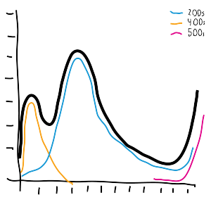
Multimodal statistics abound in real world data: multiple peaks or multiple distributions packed into a single dataset. Consider response times from an HTTP service:

• Successful requests (200s) have a "normal" latency.

• Client failures (400s) complete quickly, as little work can be done with invalid requests.

• Server errors (500s) can either be very quick (backend down) or very slow (timeouts).

Here we can assume that we have several curves overlaid, with 3 obvious peaks. This exaggerated graph makes it clear that maintaining a single set of summary statistics can do the data great injustice. Two peaks really narrows down the field of effective statistical techniques, and three or more will present a real challenge. There are times when you will want to discover and track datasets separately for more meaningful analysis. Other times it makes more sense to bite the bullet and leave the data mixed.

Time-series statistics transforms measurements by contextualizing them into a single, near-universal dimension: time intervals. At PayPal, time series are used all over, from per-minute transaction and error rates sent toOpenTSDB, to the Python team’s homegrown $PYPL Pandas stock price analysis. Not all data makes sense as a time series. It may be easy to implement certain algorithms over time series streams, but be careful about overapplication. Time-bucketing contorts the data, leading to fewer ways to safely combine samples and more shadows of misleading correlations.

Moving metrics, sometimes called rolling or windowed metrics, are another powerful class of calculation that can combine measurement and time. For instance, the exponentially-weighted moving average (EWMA), famously used by UNIX for its load averages:

$ uptime 10:53PM up 378 days, 1:01, 3 users, load average: 1.37, 0.22, 0.14

This output packs a lot of information into a small space, and is very cheap to track, but it takes some knowledge and understanding to interpret correctly. EWMA is simultaneously familiar and nuanced. It’s fun to consider whether you want time series-style discete buckets or the continuous window of a moving statistic. For instance, do you want the counts for yesterday, or the past 24 hours? Do you want the previous hour or the last 60 minutes? Based on the questions people ask about our applications, PayPal Python services keep few moving metrics, and generally use a lot more time series.

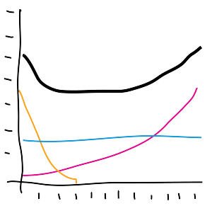
Even a little survival modeling will make your code cleaner.

Survival analysis is used to analyze the lifetimes of system components, and must make an appearance in any engineering article about reliability. Invaluable for simulations and post-mortem investigations, even a basic understanding of the bathtub curve can provide insight into lifespans of running processes. Failures are rooted in causes at the beginning, middle, and end of expected lifetime, which when overlaid, create a bathtub aggregate curve. When the software industry gets to a point where it leverages this analysis as much as the hardware industry, the technology world will undoubtedly have become a cleaner place.

https://www.paypal-engineering.com/2016/04/11/statistics-for-software/