2. Differential expression analysis - nuriagaralon/genome-analysis GitHub Wiki
Leptospirillum ferriphilum was cultured in two different ways: in a chemostat with ferrous iron (Fe2+) or in a batch leaching culture with chalcopyrite (CuFeS2). The transcriptome was obtained from three chemostat cultures and two leaching cultures, which were sequenced using Illumina HiSeq2500 obtaining paired-read data. There are a total of 10 runs available on SRA, with two files per run since it is paired-end data; and two runs per each of the 5 experiments or BioSamples, which we assume to be sequencing replicates from the same transcriptome.
The first step of this analysis is also to check the quality of the reads and trim them. The quality checks were conducted with FastQC and summarised with MultiQC, both before and after trimming. The trimming step was conducted with Trimmomatic.
FastQC was ran on the raw RNA data to see the overall quality of the reads. The following code was used, which can also be found here.
fastqc -t 4\
 -o ~/genome-analysis/analyses/02_diff_expression/01_qc_fastqc \
 -d ~/genome-analysis/analyses/02_diff_expression/01_qc_fastqc \
~/genome-analysis/data/RNA_raw_data/*.fastq.gz
The -t flag indicates the number of threads, while -o and -d indicate the output directory for the logs and final quality assessment. Each of the raw data files got a quality report, which can be found here.
The output from FastQC was difficult to analyse as there is a report file for each of the sequencing runs. Thus, the output folder was passed to MultiQC to gather all the reports into one. For this, it was only needed to navigate to the folder in question, 01_qc_fastqc, and run multiqc .. The full combined report can be found here, and the relevant plots will be analysed below.
Table 1: General statistics in raw reads
| Sample Name | % Dups | % GC | M Seqs | Sample Name | % Dups | % GC | M Seqs |
|---|---|---|---|---|---|---|---|
| ERR2036629_1 | 96.3% | 56% | 24.3 | ERR2117288_1 | 96.3% | 56% | 24.3 |
| ERR2036629_2 | 95.8% | 56% | 24.3 | ERR2117288_2 | 95.8% | 56% | 24.3 |
| ERR2036630_1 | 96.8% | 56% | 25.2 | ERR2117289_1 | 96.8% | 56% | 25.2 |
| ERR2036630_2 | 96.1% | 56% | 25.2 | ERR2117289_2 | 96.1% | 56% | 25.2 |
| ERR2036631_1 | 82.5% | 52% | 20.6 | ERR2117290_1 | 82.5% | 52% | 20.6 |
| ERR2036631_2 | 81.7% | 52% | 20.6 | ERR2117290_2 | 81.7% | 52% | 20.6 |
| ERR2036632_1 | 87.9% | 52% | 27.1 | ERR2117291_1 | 87.9% | 52% | 27.1 |
| ERR2036632_2 | 87.3% | 51% | 27.1 | ERR2117291_2 | 87.3% | 51% | 27.1 |
| ERR2036633_1 | 96.7% | 56% | 24.9 | ERR2117292_1 | 96.7% | 56% | 24.9 |
| ERR2036633_2 | 96.1% | 56% | 24.9 | ERR2117292_2 | 96.1% | 56% | 24.9 |
In Table 1, we can see the general statistics. The replicates were placed side by side for better comparison. As we can see, the replicates have the same values for all the general statistics, which is suspicious. Even if the replicates originate from the same transcriptome, the different sequencing experiment should introduce some variation.
In the general statistics which we can see at Table 1, it can be seen how the runs from continuous culture and the ones from mineral cultures have different GC and duplicate content, with the mineral being around 51-52% GC and the continuous culture at 56% GC. It could be that the transcriptomes differ in GC content because different genes are expressed, or that there is some contamination from other bacteria. This difference can also be seen in Image 1.
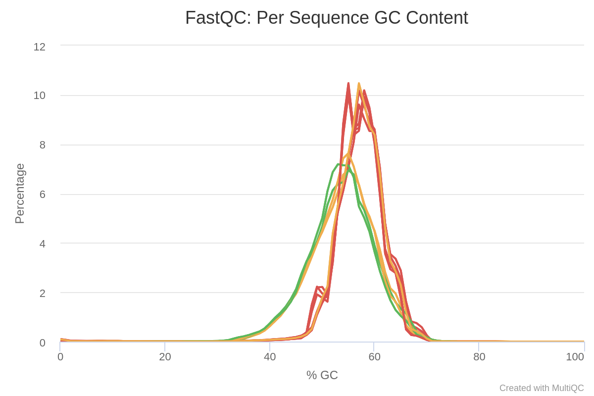
Image 1: GC content per run in raw reads
In Image 2, we can see the duplication levels in the sequences. This is normal and expected from this type of data as sequencing depth is needed to detect less expressed transcripts.
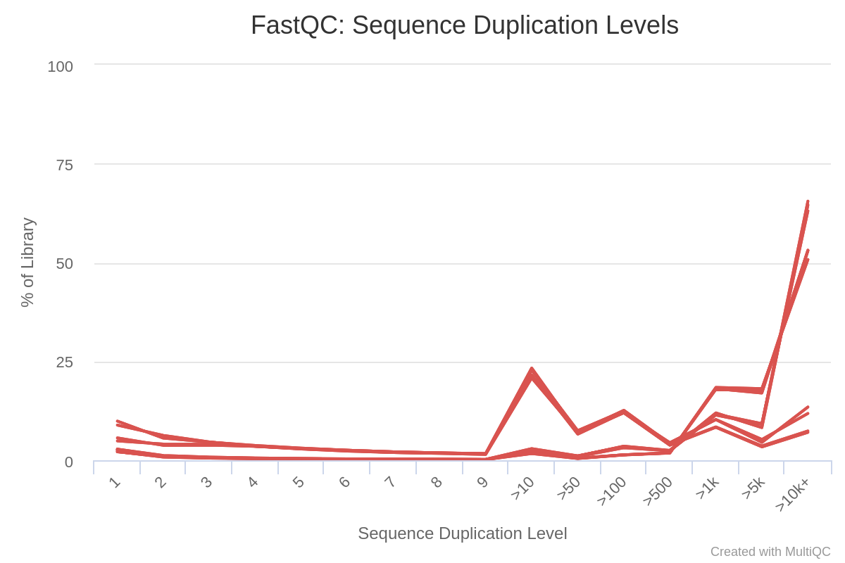
Image 2: Duplication levels per run in raw reads
In Image 3, we can see the average quality per position in the reads, in the runs. We can see how a lot of the runs have reads with low Phred score towards the beginning and the end of the reads. These are probably going to be trimmed in the next step, so it is not a problem.
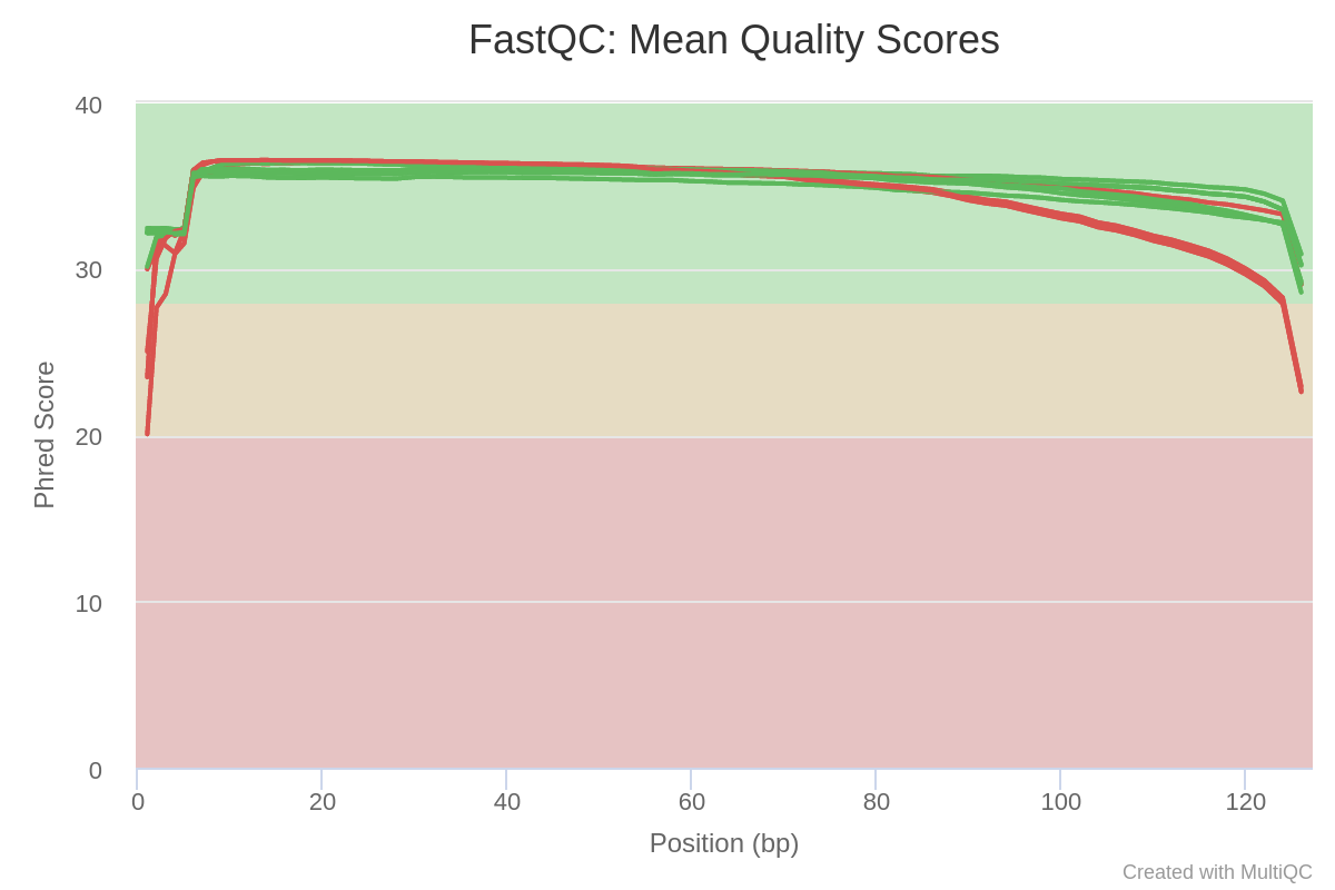
Image 3: Sequence quality per base in each run of the raw reads
Then, we can see in Image 4 that there is a lot of adapter content. These are known sequences, which will be trimmed in the next step.
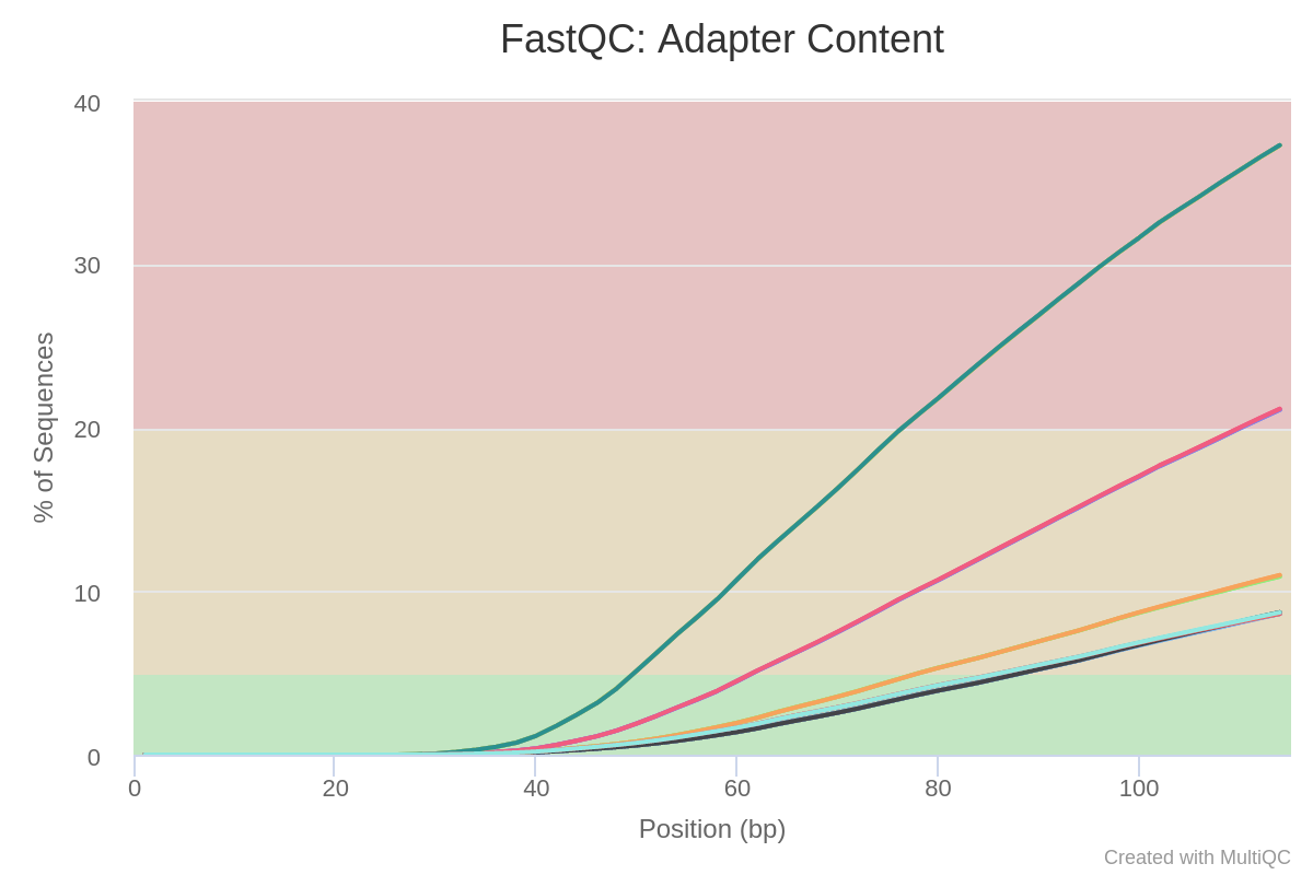
Image 4: Adapter content per run in raw reads
The RNA reads were trimmed with Trimmomatic to improve their quality. Trimmed data was available, but we conducted trimming in ERR2036629_1.fastq.gz and their paired reads ERR2036629_2.fastq.gz to check how the program worked. The following code was used to run Trimmomatic, and it can also be found here.
java -jar $TRIMMOMATIC_HOME/trimmomatic.jar \
PE -threads 4 -phred33 \
-basein ~/genome-analysis/data/RNA_raw_data/ERR2036629_1.fastq.gz \
-baseout ~/genome-analysis/analyses/02_diff_expression/02_preproc_trimmomatic/ERR2036629_Trimmed.fastq.gz \
ILLUMINACLIP:$TRIMMOMATIC_HOME/adapters/TruSeq3-PE.fa:2:30:10 \
LEADING:20 \
TRAILING:20 \
SLIDINGWINDOW:1:3 \
MINLEN:40 \
MAXINFO:40:0.5 \
The second line indicates the paired end mode, the amount of threads and that the data is encoded with phred33, which is what Illumina sequencers output. -basein and -baseout indicate the input and output files, respectively, where the reverse reads file is detected by naming similarity and three output files are generated with different suffixes (1P, 2P, 1U, 2U; paired reads and reads left unpaired). ILLUMINACLIP indicates which adapters are present on the data, which is detailed on the paper here. The conditions for LEADING, TRAILING, SLIDINGWINDOW, MINLEN and MAXINFO were set the same as the used in the article, as was found here.
In the log file for the trimming process, the following output was found:
Input Read Pairs: 24278349
Both Surviving: 21793091 (89.76%)
Forward Only Surviving: 2433801 (10.02%)
Reverse Only Surviving: 10914 (0.04%)
Dropped: 40543 (0.17%)
This shows that the majority of the reads were of good quality that could be kept.
FastQC was run after trimming as well, in both the reads that were already trimmed (with this code) and the ones trimmed in the previous step (with this code). After passing both output folders through MultiQC, there were no differences in the quality or the overall results for the reads trimmed in the previous step and the corresponding reads already trimmed. I thus decided to use the already trimmed reads to save time and memory, and therefore the quality reports from these reads will be analysed. The full combined reports can be found here for the reads trimmed in the previous step and here for the reads used for the following steps.
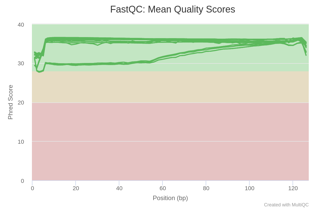
Image 5: Sequence quality per base in each run of the trimmed reads
The plots which found significant differences are found in Image 5 and 6. In image 5, we can see how the quality along the read is in acceptable phred score values, all of them over 28.
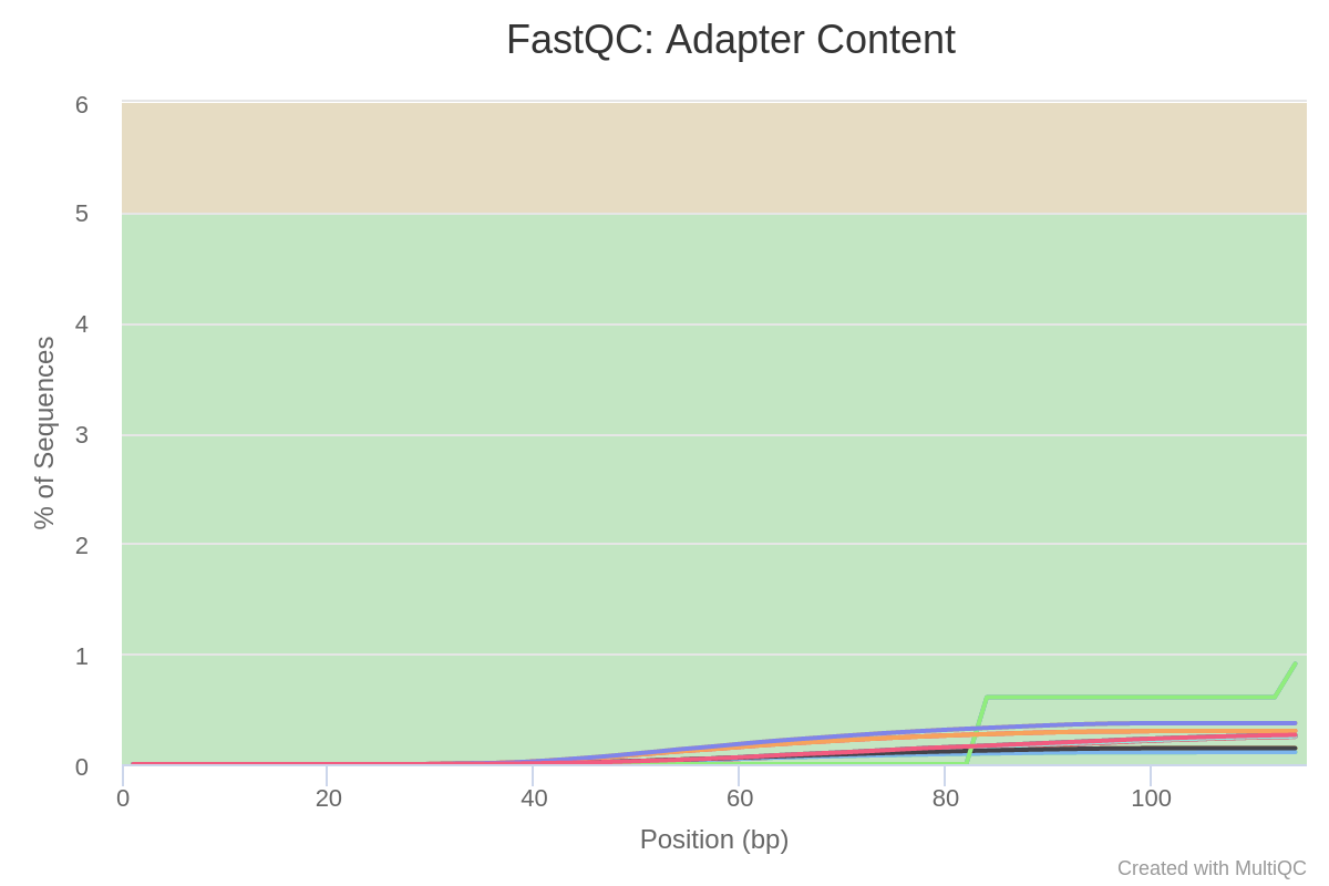
Image 6: Adapter content per run in trimmed reads
In Image 6, we can see how the adapters have been successfully trimmed from the reads. Therefore, all the sequences in these datasets should correspond to actual transcripts.
Once the reads are of good enough quality, the next step is to map them to the reference genome, i.e. the genome that was assembled previously (see Genome assembly). For this purpose, the Burrows-Wheeler Alignment tool (BWA) was used. This software maps low-divergent sequences like transcriptomic reads against a reference genome. The BWA-MEM algorithm was chosen among the three algorithms contained in BWA as it is fast, accurate and has the best performance for short Illumina reads.
The first step is to create an index for the reference genome and then run the algorithm for each pair of files with paired reads. The result, a SAM file, was directly piped into samtools, converted to a BAM file and sorted so that the alignments are in genome order. The following code, which can also be found here, was used to acquire this BAM file:
bwa index $REF -p lferrdb

for F in ERR2036629 ERR2036630 ERR2036631 ERR2036632 ERR2036633 \
ERR2117288 ERR2117289 ERR2117290 ERR2117291 ERR2117292
do
bwa mem -t 4 lferrdb \
$TRIMREADS${F}_P1.trim.fastq.gz $TRIMREADS${F}_P2.trim.fastq.gz |
samtools view -S -b | samtools sort -o ${F}.sorted.bam
done
$REF is the file with the assembled genome, and -p indicates the name of the indexed file, which is then used in the mem command. -t corresponds to the threads used by the application. The view -S -b command and flags indicate that the input is a sam file and the output should be a bam file, which is then sorted in genome order by sort -o.
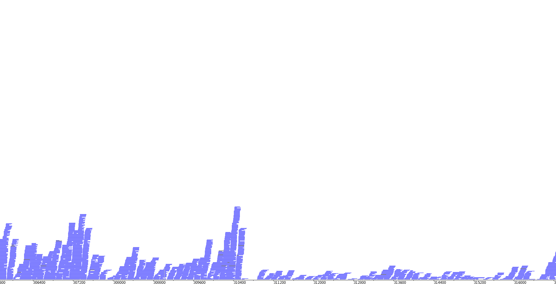
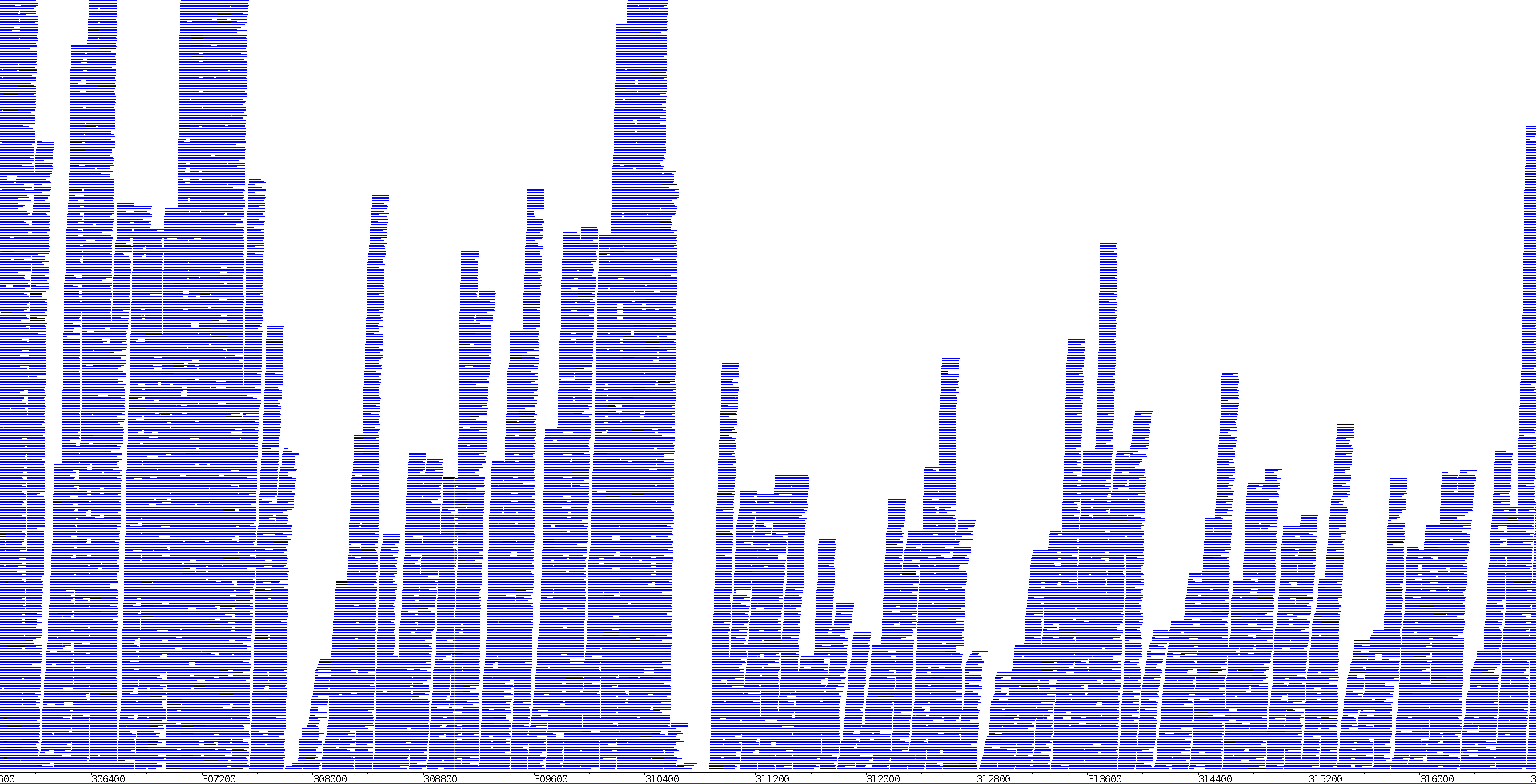
In order to visualise how the mapped reads look in the genome, the BAM files were loaded together with the assembled genome in Artemis BamView. A snapshot of this visualisation can be seen in Image 7 for a chemostat sample and in Image 8 for a bioleaching sample.
 |
 |
|---|---|
| Image 7: Visualisation of ERR2036629 RNAseq reads in Artemis | Image 8: Visualisation of ERR2036631 RNAseq reads in Artemis |
As we can see, within the same genome, there are regions with more read coverage and regions with less. This is consistent with the fact that there is more coverage for features that are highly expressed than for features which have low expression. The two images show the same region of the genome but clear differences can be seen between them. The first instinct would be to attribute this to a change in expression between the two conditions for these certain genes, which might be possible. However, it should be taken into account that this is raw data and it is therefore not standardised, so some of the differences are likely due to one of the two sequencing experiments producing more total reads.
Afterwards, we wanted to evaluate the quality of the mapping steps. For this, samtools was used with the following code, also found here.
for F in ERR2036629 ERR2036630 ERR2036631 ERR2036632 ERR2036633 \
ERR2117288 ERR2117289 ERR2117290 ERR2117291 ERR2117292
do
mkdir $F
cd $F
samtools stats ../../05_mapping_bwa/${F}.sorted.bam > ${F}.stats
plot-bamstats -p $F ${F}.stats
cd ..
done
The output of this analysis is a folder for each of the samples with plots illustrating various characteristics. We focused on the amount of reads that mapped successfully to the genome. For this, we extracted the relevant information from each stats file using grep, piped it here and analysed it using R with this script. The result can be found here, and a summary can be found in Table 2.
Table 2: Reads that map back to the genome
| Sample | % of reads mapped | Sample | % of reads mapped |
|---|---|---|---|
| ERR2036629 | 99.5306 | ERR2117288 | 99.5306 |
| ERR2036630 | 99.5553 | ERR2117289 | 99.5553 |
| ERR2036631 | 69.4599 | ERR2117290 | 69.4599 |
| ERR2036632 | 71.6470 | ERR2117291 | 71.6470 |
| ERR2036633 | 99.7318 | ERR2117292 | 99.7318 |
As we can see in Table 2, the chemostat cultures have over 99% of the reads mapping back to the genome, while the mineral cultures have around 70%. This could be due to some contamination in the mineral cultures, which would mean that it contains sequences that do not correspond to L. ferriphilum and thus do not map to its genome.
We can also see that, again, the replicates have the exact same value among themselves. This data, together with the data in Table 1, make us suspect that the technical replicates contain the same data. To inspect this, a python script which compared if the read sequences were the same was ran using this script. The results can be found here, which shows that the technical replicates have the exact same information. Thus, from now on, only the files starting with ERR203 will be used for further analysis.
After mapping the genes to the genome, the next step is to count how many reads map to each of the annotated features. For this, there exist various software such as the featureCounts package for R and HTSeq. The latter was used because it is a computationally heavy job and it is installed in UPPMAX. The following code was used to conduct read counting, and it can also be found here.
for F in ERR2036629 ERR2036630 ERR2036631 ERR2036632 ERR2036633
do
htseq-count -f bam -r pos -s reverse -t CDS -i ID \
$BAM${F}.sorted.bam lferr_nofasta.gff > ${F}.txt
done
The -f flag indicates the format of the input data, -r pos is used because the input data was sorted in position order from the genome, -s reverse because of how the data was generated, with Illumina TruSeq Stranded total kit, as seen in the paper by Christel et. al. -t determines the type of feature that will be counted, and -i indicates the column to be used as a feature ID. The output is a text file for each of the samples which contains a list of the CDS features and how many reads map to each of them in tab-separated values.
At the end of the file, we also find the reads that do not map to any feature. Using this R script, Table 3 was constructed.
Table 3: Summary of the mapping and counting steps
| Sample | % of reads mapped | % of total to gene | % of good q to gene | % of good q to no feature |
|---|---|---|---|---|
| ERR2036629 | 99.5306104122632 | 4.59912203190424 | 48.9562087320112 | 37.4646638859447 |
| ERR2036630 | 99.5553171825923 | 3.02037966281405 | 40.3041978971555 | 48.4387524032552 |
| ERR2036631 | 69.4599179372571 | 35.0598030416105 | 36.1545931578991 | 9.86107283408137 |
| ERR2036632 | 71.6470991648541 | 36.2832023441735 | 37.6865833571787 | 12.0382949918397 |
| ERR2036633 | 99.7318854495836 | 3.88027365730577 | 46.5115246899585 | 44.5761446618098 |
As we can see in the third column of Table 3, the amount of reads that map to genes is very low in the chemostat cultures. However, by inspecting the HTSeq output, there were a large part of the reads that were deemed to be of too low mapping quality and were excluded from the mapping. Adjusting the number of total reads using this factor, we can see that all samples map around 40% of their reads to features. The reads which were of low quality were probably reads that mapped to rRNA genes, as there are multiple copies of these genes in the genome and they can only be ambiguously mapped. The other 60% likely corresponds to expressed RNA that is not CDS, such as tRNAs or small RNAs.
Differential expression analysis was conducted to see the differences in the expression of different genes between the two different conditions of the cultures: chemostat and bioleaching. With this, we can find which genes are expressed differently in the two conditions and to what extent. There are many R packages which can be used for this type of analysis, such as EdgeR, Limma and DESeq2. Limma is not good for experiments with few replicates, like this project. In the end, DESeq2 was used, and the script which conducted the analysis and created the differential expression plots can be found here.
First, the data was formatted according to what DESeq2 needs for the analysis; which consists on having the loci as row names and the counts from each experiment as columns, with the experiment name as the column name. This can be seen in Table 4. It also requires the metadata to know which two types of cultures there are and perform the differential expression, which can be seen in Table 5. Then, the analysis is conducted on this data set and different plots are drawn.
Table 4: Head of the counts data table
| ERR2036629 | ERR2036630 | ERR2036631 | ERR2036632 | ERR2036632 | |
|---|---|---|---|---|---|
| LFT_00001 | 432 | 348 | 3763 | 5276 | 463 |
| LFT_00002 | 400 | 310 | 4703 | 5488 | 384 |
| LFT_00003 | 1052 | 579 | 6894 | 7604 | 789 |
| LFT_00004 | 551 | 273 | 2974 | 2574 | 338 |
Table 5: Culture metadata. Also found here
| Alias | Type | |
|---|---|---|
| ERR2036629 | LNU-LXX9-Si00-CnA-P-B7-R1 | Chemostat |
| ERR2036630 | LNU-LXX9-Si00-CnA-P-B1-R1 | Chemostat |
| ERR2036631 | LNU-LXX-Si00-14B-P-R1 | Mineral |
| ERR2036632 | LNU-LXX-Si00-14C-P-R1 | Mineral |
| ERR2036633 | LNU-LXX9-Si00-CnA-P-B6-R1 | Chemostat |
Afterwards, the differential expression analysis was conducted. In the following code, Tables 4 and 5 are used to construct the data object. Then, with the type of culture as the contrast, the differential expression is analysed.
# Create DESeq data object
dds <- DESeqDataSetFromMatrix(
  countData = filtered_dataset,
  colData = metadata,
  design = ~ Type
)

# Conduct DESeq analysis
dds <- DESeq(dds)
resAll <- results(dds)
res <- results(dds, contrast = c("Type","Chemostat","Mineral"))
Afterwards, different summary plots can be constructed from the dds dataset or the res results.

Image 8: PCA of the variance in expression.
In Image 8, a principal component analysis of the different samples is shown. The plot was constructed using the plotPCA function from the DESeq2 R package. In this plot, the principal component axes represent the variance in difference in expression in all the genes collectively. As we can see, the chemostat and mineral cultures are clustered to the left and right of the plot, respectively. Samples from the same culture type are quite separated in the PC2 axis, but this one only expresses a 9% of variance in differential expression, while PC1 expresses an 87%. Therefore, this plot shows that there is a difference in gene expression between these two states, which probably relates to genes that are needed in one environment and not so much in the other.
Nevertheless, just from a PCA plot it cannot be known which are the genes specifically that are differentially expressed. Consequently, a volcano plot was constructed using the Enhanced volcano R package, which can be seen in Image 9.
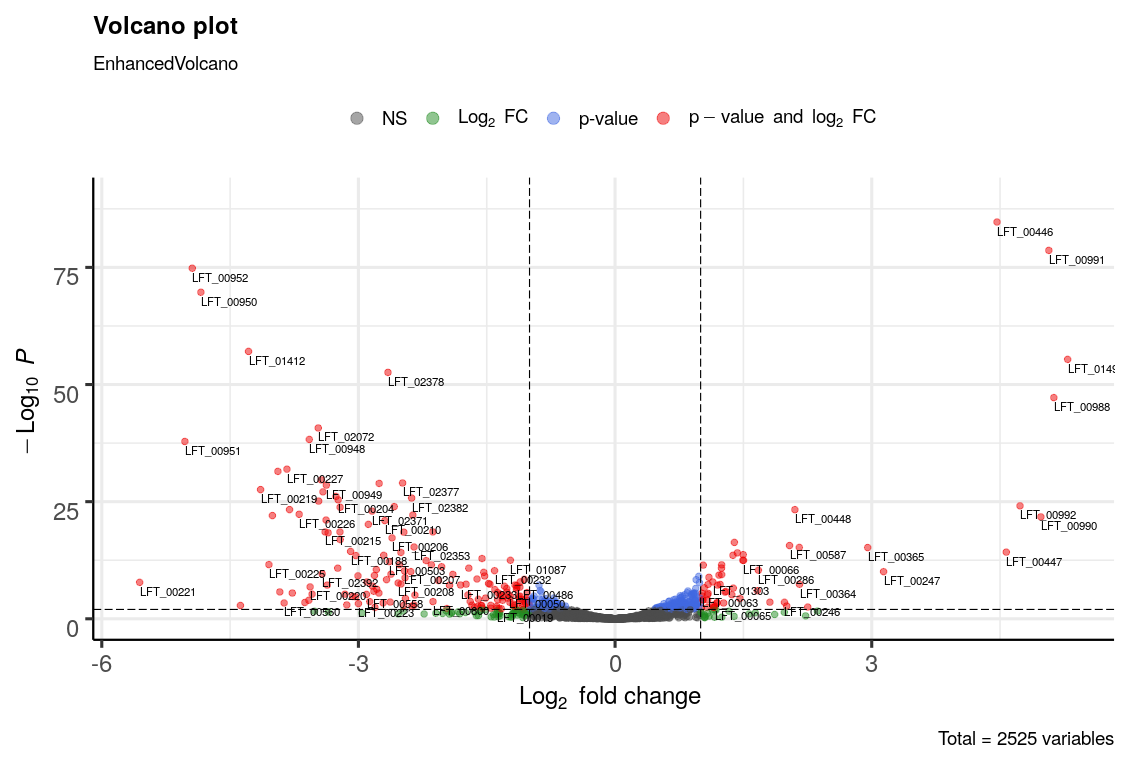
Image 9: Volcano plot of the differential expression
This plot shows the p-value and the fold change of the different genes between the two types of cultures. The p-value is a measure of how probable it is that the change in the amount of reads for each locus between the types of samples is due to a biological difference instead of just chance; and the fold change measures the magnitude of this difference. Of course, the greater the magnitude, the less likely it is that it occurred by chance, so a larger fold change is correlated to a more significant p-value.
In Image 9, the p-value cutoff was set as 0.01. Even then, there were quite a lot of genes with significant p-value and fold changes, which makes it difficult to interpret. It can be seen, however, how more genes are clustered towards the negative values of fold change, which means that a lot of the genes are more expressed in mineral cultures.
In order to find which are the genes with more significant changes, a heatmap of expression of the most significant genes was constructed. Moreover, an overview of differential expression between both sample types according to their function was also constructed. In these latter plot, the loci are assigned a functional category according to their annotation, and thus we can see which of the categories have genes that are differentially expressed and which do not. This plot might give an insight into what kinds of genes are required in one culture over the other.
Ideally, we would want to assign these categories manually, which would make it more worthwhile to compare the results of this plot against the one in the article. There was, nevertheless, not enough time for this, so the information from the article was used instead. To this end, a pairwise BLAST was run between the article loci and the project's loci, which is shown in the code below. The full code can be found here.
# make database
makeblastdb -in ../../01_genome_assembly/09_annotation_prokka/lferr.faa -dbtype prot -out lferr_prot -parse_seqids

# Run blast and reformat
blastp -db lferr_prot \
-query ../../../data/reference/lf_merged.faa \
-out proteinclassif.txt \
-num_threads 2 -outfmt 11

blast_formatter -archive proteinclassif.txt -outfmt 6 -out proteinclassif_tab.txt
A database was constructed which contained the project's loci. Then, the pairwase BLAST was run and the results were outputted in the tabulated format, as the first two columns would contain pairs between the project loci with the article loci.
Making use of this table, where each locus in the article was associated to one functional category; and this table, where each specific functional category was linked to a more general group according to the Supplemental File 1 of the article, each locus was assigned a functional category. Two additional general categories were added, Cytochromes and Nitrogen fixation, as it might show interesting results and they do not fully fit into any of Christel et. al's categories.
Together with the information from annotation refinement, each locus can be associated to a gene name (except for the hypothetical proteins), a specific functional category and a general functional category. This information, together with the DESeq2 results, were used to create the plots shown in Images 10 and 11.
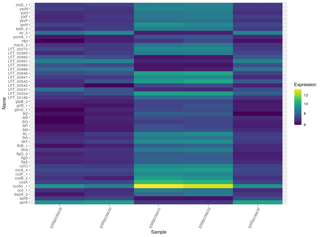
Image 10: Heat map of most significantly differentially expressed genes.
In Image 10, we can see a heat map which contains those genes with a log FC larger than 3 (in absolute values) and an adjusted p-value lower than 0.001. The cutoff for the p-value is more stringent than for Images 9 and 11, mainly because with a looser p-value there were too many significant genes to interpret. Moreover, these are the genes that present the clearest differences between chemostat and bioleaching cultures, so they should give an insight as to where the biggest differences lie.
In this table we can find these loci tied to their general function. As we can see, most correspond to motility. They also correspond to polysaccharide synthesis, metal resistance, cytochrome genes, oxidative stress response and nitrogen fixation. Moreover, bioleaching cultures seem to have a higher expression in general, at least for most of the genes in the heatmap.
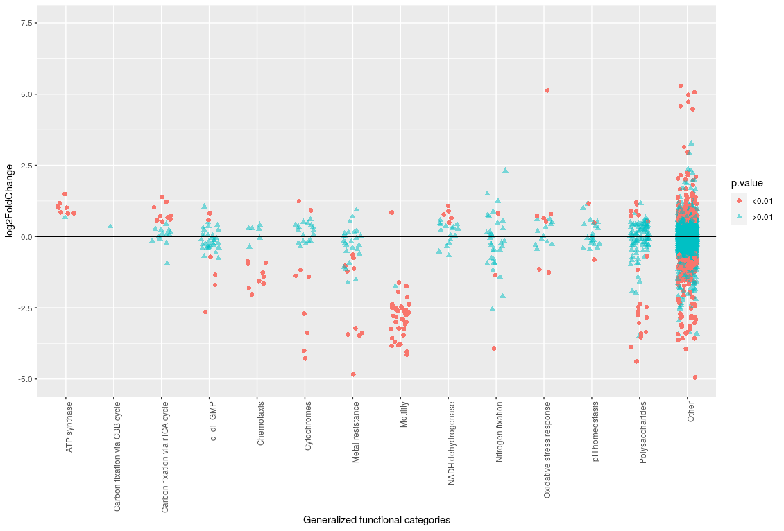
Image 11: Differential expression by functional type
In Image 11, we can see how practically all motility genes are differentially expressed with a significant p-value and large fold change. In this plot, a positive log2FoldChange means that there is a higher expression in chemostat cultures and viceversa. Thus, motility genes are more expressed in mineral bioleaching cultures. Some chemotaxis genes also have increased expression in a bioleaching environment, as well as metal resistance and polysaccharide synthesis genes.

Image 12: Differential expression by functional type, from Christel et al. Both RNA and protein expression are present in this plot, but only the RNA data will be used for comparison
All these are coherent with the information from the article in Image 12. L. ferriphilum in bioleaching cultures would attach to the mineral, thus making use of the motility and chemotaxis genes; as well as metal resistance. The metal resistance genes present in the heatmap in Image 10 are mostly copper efflux proteins, which is consistent as chalcopyrite (CuFeS2), the bioleached mineral, contains copper.
L. ferriphilum in bioleaching cultures would also form biofilms, which explains the increase in expression for some polysaccharide related genes. It is mentioned by Christel et al. that the expression of these biofilm genes might have been higher if the cells from the biofilms themselves were the ones sequenced instead of the cells in the supernatant medium.
It is interesting how some cytochrome related genes have an increased expression in bioleaching cultures. This seems to be related to a change in stress conditions (Paulino et al. 2002, Galleguillos et al. 2008), probably the same which caused an increase in expression for metal resistance genes. In the article it is mentioned that nitrogen fixation, oxidative stress response and pH homeostasis genes were not too affected by the change due to the controlled conditions of the experiment. If the bioleaching cultures had been exposed to more environmental stress, we might have seen changes in the expression of these genes, and maybe even more changes in the cytochromes.
Other cytochrome genes, however, together with ATP synthase related genes, have higher expressions in chemostat cultures. According to Christel et al., this might be due to a shift towards NADH formation instead of proton motive force. This is, however, not observed in NADH dehydrogenase genes, in neither the article nor this project.
Leptospirillum ferriphilum has an interesting metabolism due to its uncommon niche. Thus, KEGG Mapper was used to map the metabolic pathways and other functions. For this, an R script was written to extract the KEGG orthology numbers from the eggNOG-mapper output.
Afterwards, the KO numbers were submitted to the online server off KEGG Mapper. The output consisted in various pathway maps which have the genes that were present in the input highlighted. There were too many maps to discuss, so only the most complete or interesting ones will be discussed. The full results, detailing which loci correspond to which path, can be found here.
In Image 13 we can see the pathway for Nitrogen metabolism. Even though many of the genes are not present (likely due to them not having KO number in the annotation), we can see how the Nif genes responsible for nitrogen fixation are present. This is consistent with the information from the article.

Image 13: Nitrogen metabolism KEGG pathway. The genes highlighted in green are present in the input.
Another interesting characteristic of L. ferriphilum is its ability to form biofilms. As can be seen in Images 14 to 16, L. ferriphilum has many genes that correspond to three different biofilm pathways. The pel operon from Pseudomonas aeruginosa, for example, is almost present in its entirety, as can be seen in Image 14. The genes for glycogen biosynthesis are also all almost present, as can be seen in Image 15.

Image 14: Biofilm formation in Pseudomonas aeruginosa KEGG pathway.

Image 15: Biofilm formation in Escherichia coli KEGG pathway.

Image 16: Biofilm formation in Vibrio cholerae KEGG pathway.
Furthermore, in Image 16 we can see some polysaccharide synthesis genes that contribute towards flagellar assembly. As seen before, motility genes are very expressed in bioleaching cultures, and flagella are an important aspect for the motility of L. ferriphilum. As can be seen in Image 17, almost all genes for flagellar assembly were detected. Another important aspect for motility is chemotaxis, as it directs the bacteria where they should go. As can be seen in Image 18, many of these genes are also present. Looking closely, we can see how chemotaxis genes activate the flagellar assembly, and genes such as FliG, FliM and FliN which form the C ring are found in both pathways, effectively connecting chemotaxis with the assembly of flagella.
 |
 |
|---|---|
| Image 17: Flagellar assembly KEGG pathway | Image 18: Chemotaxis KEGG pathway |
Comparative genomics are a useful tool to find whether different genes are present in more than one species or not. Acidithiobacillus ferrooxidans is another gramnegative bacteria which is used for the bioleaching of copper (Valdés et al. 2008). Thus, it might be interesting to see whether it shares genes with L. ferriphilum or not, in spite of belonging to different phylums.
A BLAST search was conducted comparing the annotated proteins of L. ferriphilum with the proteins from A. ferrooxidans, from the RefSeq database. The full code can be found here.
# make database
makeblastdb -in ../../01_genome_assembly/09_annotation_prokka/lferr.faa -dbtype prot -out lferr_prot -parse_seqids

# Run blast and reformat
blastp -db lferr_prot \
-query aferr.faa \
-out compgen.txt \
-max_target_seqs 1 \
-num_threads 2 -outfmt 6\
It is similar to the BLAST conducted for the category assignment in the Differential Expression Analysis, but with -max_target_seqs set to 1, to get only the best hits. Afterwards with this R script, the results were filtered to keep only those with e-values inferior to 10-5.
From the 2525 CDS in L. ferriphilum, 907 yielded good hits in the pairwise blast. Of these, only 279 are present with the same annotation. However, the vast majority are ones where the gene name is empty in either of the species, and rarely are there annotations which are different. The full comparison file can be found here.
The genes which are common in both species are, for example, housekeeping bacterial genes such as the ones related to replication or transcription. Other genes such as copper efflux genes are also present in both species, which confirms that they have similar "nonessential" genes due to their shared niche.