Genome Assembly

The Leptospirillum ferriphilum type strain genomic DNA was sequenced using two PacBio SMRT cells, which yielded raw long read data. The first step would be to check the quality of these reads and trim them. One option would be to use FastQC to check for quality. However, Canu, the assembler that will be used, can also be used for quality checks; and it also has a trimming step. Therefore, we directly used the raw reads to run Canu, with the following code, also available here. This command calls the Canu pipeline which contains three phases: correction, trimming and assembly, and keeps the outputs from each step.

canu \
 -p lferriphilum -d $OUTPUT \
 genomeSize=2.6m stopOnReadQuality=false maxThreads=4 \
 -pacbio-raw $INPUT

The -p flag indicates the prefix that the output files will have, which will be sent to the -d directory. maxThreads indicates the maximum number of processors that can be used. Together with genomeSize, which indicates the estimated size of the genome that will be assembled, Canu will estimate the resources needed and how the jobs will run. -pacbio-raw indicates the type of raw reads, and $INPUT is the file or files with said reads. stopOnReadQuality was set as false because the quality of the reads is not as optimal as it would be expected. The rest of the parameters are set as default.

The assembly produced four different contigs:

Contig	Alternate name	Coverage	Size (pb)
tig00000059	tig59	75.14	48,946
tig00000061	tig61	1.35	2,597
tig00004063	tig4063	0.00	21,143
tig00004064	tig4064	5290.83	2,563,357

It seems like tig4064 contains the genome, as the size is very similar to the reference genome (2,569,357 pb); and tig59 the phage that was found by the authors, which is slightly shorter in the reference genome (41,141 pb). The coverage for both these contigs is acceptable, albeit significantly lower for tig59.

The coverages for the other two contigs are very low. By looking at the sequence for tig61, available here, it can be seen how almost all of it is G and T, with a large amount of homopolymers. This contig is probably either a region that could not be assembled or sequencing errors/contamination, likely the latter.

The sequence for tig4063, however, looks normal at first glance. Something of note is that this contig is assembled from a single, quite long read. Since it was displayed as a contig, the read probably has high quality. I wonder why it was not assembled within the genome: is it misassembled somewhere?

Assembly Evaluation

After the assembly, assessing its quality is needed to see if it had to be reassembled or rechecked. For this, various software were used. Initially, QUAST and MUMmerplot were used for this purpose. Afterwards, many dotplots were generated with Gepard.

QUAST (Quality Assessment Tool for Genome Assemblies) was used to generate a summary report of different metrics, plots of cumulative contig length, Nx and GC content, among others. An Icarus output is also generated, which displays the alignment of the contigs on the reference genome. The following code was used to run QUAST, which can also be found here.

quast.py \
~/genome-analysis/analyses/01_genome_assembly/01_assembly_canu/lferriphilum.contigs.fasta \
-R ~/genome-analysis/data/reference/lferriphilum_ref.fasta \
-o ~/genome-analysis/analyses/01_genome_assembly/02_eval_quast/ \
--gene-finding

The input file is the contigs file from the Canu assembly, and -R is the reference genome. The output directory is indicated with -o and --gene-finding for QUAST to attempt at predicting genes. However, the gene finding did not work, but we will conduct annotation afterwards so it is not a problem.

MUMmer is a tool that computes rapid alignments of entire genomes. With MUMmer, the Canu contigs file was aligned to the reference genome. Afterwards, a dot plot was computed by MUMmerplot. This was done sequentially in the same bash script, which can be found here.

mummer -mum -b -c \
$REF \ 
$INPUT \
> $MUMS/lferriphilum.mums

mummerplot \
-Q $INPUT \
-R $REF \
$MUMS/lferriphilum.mums \
--png --prefix=lferriphilum

$INPUT and $REF are the contigs and reference sequence, respectively. -mum computes the matches between the two sequences, while -b and -c are for the sequence to compute both forward and reverse complement matches, and report them relative to the query sequence. --prefix indicates the prefix of the output file, and --png its extension.

The following table is a summary report from QUAST's output. The full report can be found here.

Genome statistics	lferriphilum.contigs
Genome fraction (%)	97.566
Duplication ratio	1.015
Largest alignment	1463673
Total aligned length	2584500
NGA50	1463673
LGA50	1
Misassemblies
# misassemblies	1
Misassembled contigs length	2563357
Mismatches
# mismatches per 100 kbp	0
# indels per 100 kbp	5.89
# N's per 100 kbp	0
Statistics without reference
# contigs	4
Largest contig	2563357
Total length	2636043
Total length (>= 1000 bp)	2636043
Total length (>= 10000 bp)	2633446
Total length (>= 50000 bp)	2563357

From the report we can confirm the quality of the assembly:

• A high genome fraction value and duplication ratio close to 1 indicate that the contigs cover almost all the reference genome and they do not overlap a lot.
• The NGA50 value indicates the smallest aligned block when they cover at least half. Together with the LGA50, we can see how the value belongs to only one aligned block, i.e. is part of tig4064, as it is the only one large enough.
• We can see how we have one missassembly and various indels.

In Fig. 1 we can see how the GC content in both the contigs and the reference genome is similar. This makes sense, as both are assembled from the same pool of reads, but it could have been different if the assembler had picked different reads for the assembly. However, if we check the NCBI genome list for the Leptospirillum genus, we can see that the GC content is around 50% for all the available genomes, which is also consistent with the obtained results.

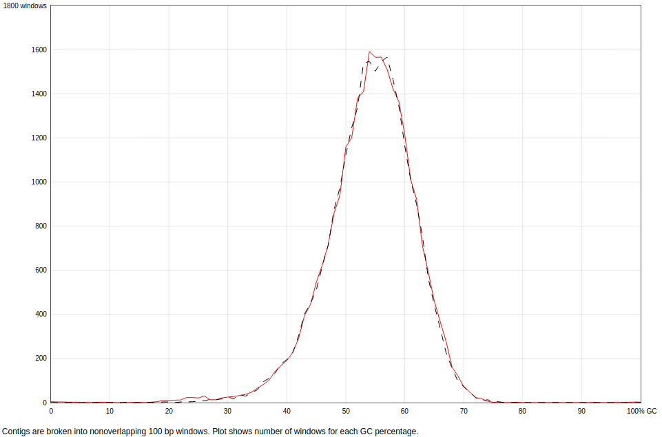
Figure 1: GC content in the contigs (red) and the reference genome (black). The plot shows the amount of 100pb windows in the sequence that have certain %GC.

Then, we looked at the Icarus visualisation tool. Here, in Fig. 2, we can see how tig4064 is completely aligned to the reference genome. We can see how the misassembly seems to be a relocation of part of tig4064. We can also see how tig4063 is aligned between the end and the beginning of tig4064, and tig4064 overlaps with itself. We see how there is a gap that is not present in our contigs, but is present in the reference genome. This is both ~20kbp of genomic sequence and the entire phage.

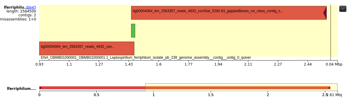Figure 2: Visualisation of the contigs aligned to the reference genome. The reference genome is the black ruler with the base pairs, while tig4064 is represented in red and tig4063 in green.

In Fig. 3 we can see the dot plot generated by MUMmerplot. A perfect alignment would be shown as a red diagonal line. The shown pattern indicates a relocation, which is in consensus with the information from QUAST. We can also see how the reverse complementary of the phage matches part of the genome, which was mentioned by Christel et al..

Figure 3: MUMmer dot plot of the assembly (y) vs the reference genome (x). In red are represented the forward matches and in blue the reverse matches.

Afterwards, we attempted to get more dot plots using Gepard. In Fig. 4 we see the figure that would correspond to the same plot as MUMmerplot. We can see how the plot is the same, and the difference in the plot is because the reference sequence is on top instead of the bottom, so the lines are inverted. It could also be seen in Fig. 3, but in Fig. 4 it is clear how the first contigs of our assembly, which are the top part of the y axis, do not correspond to any sequence in the reference genome.

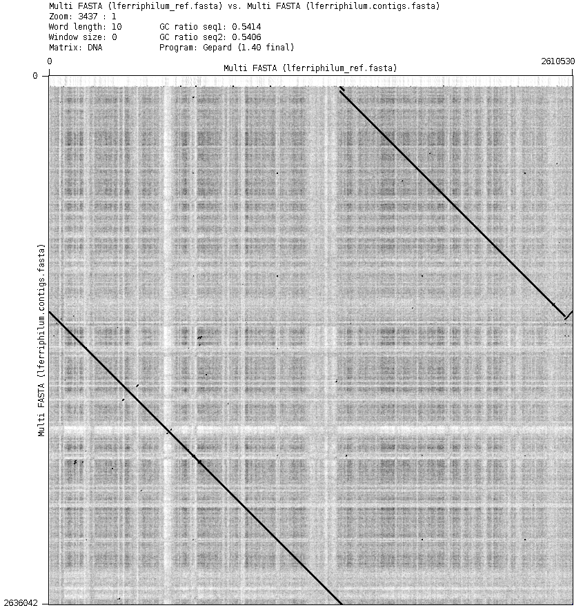
Figure 4: Gepard dot plot of the assembly (y) vs the reference genome (x).

In Fig. 2 to 4 there are various characteristics of interest that we will look further into:

• The misassembly or relocation (Fig. 2-4)
• The overlap of the beginning and end of tig4064 (Fig. 2-4) and tig4063 in the same region (Fig. 2, and also 3 and 4 but less clearly. Specially in Fig. 4, a line in the top middle of the plot is separated from the line of tig4064, which is tig4063 and this overlap.)
• The phage contig missing from the assembly (Fig. 2)
• The contig suspected to be a phage does not match with any of the reference sequence (Fig. 3, 4)
• The gap in the assembly (Fig. 2)

Misassembly and overlap

The misassembly is clear in both dot plots and the Icarus display. However, Leptospirillum ferriphilum is a prokaryote, which means that it likely has a circular genome. Thus, this misassembly is explained by the fact that the arbitrary starting point of the genome has been set differently between the assembly and the reference.

The fact that the genome is indeed circular is also supported by what can be seen in Fig. 5. By looking at tig4064, we can see that the beginning and the end of this contig overlap. This could suggest that it is either a repeat or that the sequence is continuous and thus circular. By looking at tig4063 we can confirm that it is the latter, as the sequence covers the beginning and the end of tig4064 and is contiguous.

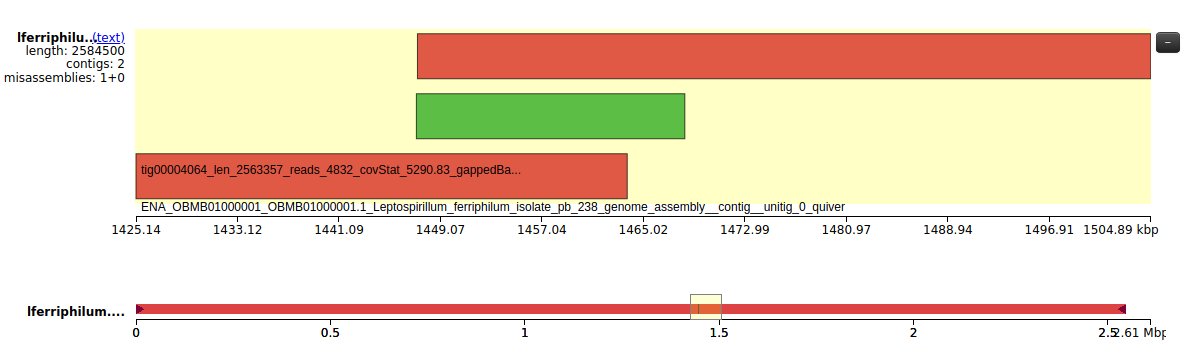
Figure 5: Visualisation of tig4064 (red) and tig4063 (green) and their overlap.

The fact that tig4064 has a repeated sequence at the beginning and end which is very likely to be inaccurate might be a problem when annotating. If there are any genes in that stretch of sequence and we try to map them to a genome with repeats, it might map some to one part and some to the other part.

There are two strategies we could adopt here. One would be to remove the repeated sequence from one of the sides. The disadvantage of this method is that a gene might be cut in half, which would make annotation and mapping of transcripts difficult. The other strategy is to recircularise the genome and set a specific start which does not cut any genes in half. It seems the better choice, so this was attempted using Circlator and can be found in the next section.

Gap in the assembly

In Fig. 2 we can see how, at the end of the reference genome, there is a part that no contigs map to, besides the phage contig. However, when we check the dot plot, these 20kb match the middle of the contig, at around 1Mbp, as can be seen in Fig. 6.

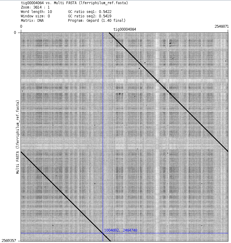
Figure 6: Dot plot of the reference genome (y) vs tig4064 (x). In blue is marked, roughly, the point from where no contigs map in Icarus anymore.

It is likely that this region is a repeated region present in the reference genome, likely similar to the repeat in the assembly which, as explained, is due to the genome being circular. This is confirmed by the fact that tig4064 in Icarus is also cut at around 1MB and then the part after it maps in the beginning of the reference genome. This can be seen in Fig. 7. It is also further confirmed by the dot plot of the reference genome vs itself, where the beginning also maps to the end of the sequence.

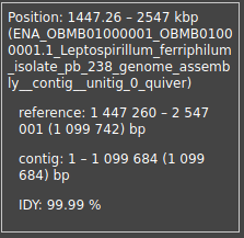
Figure 7: Mapping of tig4064 in the end of the reference genome. The contig maps until 1,083,023bp and the rest maps in the beginning.

To further confirm this, a reference vs reference dot plot was conducted.

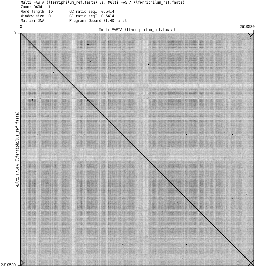
Figure 8: Dot plot of the reference genome vs the reference genome, excluding the contig with the phage. The beginning of the sequence maps to the beginning and the end of the sequence, which can be seen in the top right and bottom left corners.

Missing phage and tig59

In the reference genome there is a contig which represents a putative phage. This contig is not present in the assembly, as can be seen in Fig. 2. However, by looking at Fig. 3 and 4, it can be seen that the phage, which is at the end of the reference genome, maps in reverse to the assembly. Christel et al. mentioned in their paper that this happened in their assembly as well, where it putatively represents a prophage. Thus, in this assembly, it is likely that the assembler deemed the reads to belong exclusively to the genome and the separate contig for the phage was not obtained. Since the aim of this project does not involve the study of the phage, it is of no consequence.

Now, however, we are sure that tig59 is not the phage. It also does not match with any part of the reference in Fig. 3 and 4. A dot plot of the assembly vs the assembly was constructed, and in Fig. 9 the detail of tig59 can be seen. The pattern created by this dot plot is very unnaturally regular, so this contig is likely not biologically significant.

Figure 9: Close-up of the dot plot of the assembly vs the assembly. The regular pattern on the top left corresponds to tig59 mapping with tig59.

To confirm this, a BLAST search was conducted. blastn was used to compare tig59, our $INPUT, to the whole nucleotide database, nt_v5, and the results were recorded in the $OUTPUT directory. The following code was used for this analysis, and can also be found here.

blastn -db nt_v5 \
-query $INPUT \
-out $OUTPUT

The top hits, which can be seen in the summary, indicate that this sequence is MG551957.1. This is a synthetic PacBio control sequence and thus has no biological meaning, as was expected.

Extra: Assembly refinement

The quality of the assembly was good, but since it had an overlapping region in the beginning and the end, it seemed appropriate to attempt a circularisation of tig4064 using the Circlator pipeline. The pipeline consists of 6 consecutive steps: mapping the reads to the assembly, extracting the mapped reads, reassembly of the extracted reads using SPAdes, merge and circularisation of the contigs, and cleaning and fixing the contig start position at the dnaA gene. The reads that were corrected and trimmed and tig4064 were used as input, and Circlator was run with the following code, which can also be found here.

circlator all \
~/genome-analysis/analyses/01_genome_assembly/01_assembly_canu/contigs/tig00004064.fasta \
~/genome-analysis/analyses/01_genome_assembly/01_assembly_canu/lferriphilum.trimmedReads.fasta.gz \
~/genome-analysis/analyses/01_genome_assembly/05_circularization_circlator \
--threads=4

The final output from Circlator was a fasta file with the circularised tig4064. The log files, found here indicate that everything was completed without a problem. The gene used to fix the start of the contig was A0A094W894, which is the L. ferriphilum dnaA protein.

Evaluation

QUAST, with the code found here, was used to generate a summary report about the circlator output with respect to the reference genome.

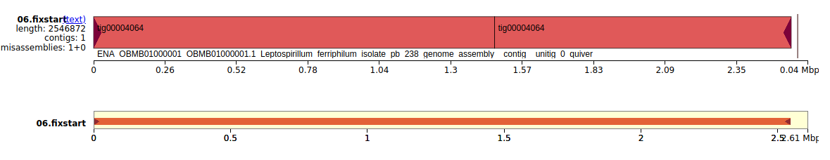
Figure 10: Visualisation of the contig aligned to the reference genome. The reference genome is the black ruler with the base pairs, while tig4064 is represented in red.

In Fig. 10 we can see that the contig has no overlaps at all, still does not have the last 20kb which is good since it was the overlapping of the assembly contig, but is still translocated with respect to the assembly genome. This is weird since Christel et al. also used Circlator to circularise the genome and fix the start to dnaA, but it seems that the overlap stayed and the beginning does not seem to be the dnaA gene. Checking the beginning of the reference fasta file showed that the contig does begin with ATG, however.

We thus constructed a Gepard dot plot to check the assembly with the reference genome, and the translocation was indeed still there, as can be seen in Fig. 11.

Figure 11: Gepard dot plot of tig4064 after circlator (y) vs the reference genome (x)

A Gepard dot plot of the contig before and after Circlator was also constructed. This plot is shown in Fig. 12, where it can be seen how the overlap disappeared, as no part of the contig from Canu mapped twice on the contig from Circlator.

Figure 12: Gepard dot plot of tig4064 (y) vs tig4064 after Circlator (x)

Afterwards, we wanted to confirm whether the first gene in both the output from Circlator and the reference genome was the dnaA gene or not. For this, a BLAST search was conducted. blastx was used to compare the beginning of both files (by obtaining the first 30 lines with head) to the refseq_protein_v5. The following code was used for the reference genome, and a similar command for the Circlator output. The full code can be found here.

blastx -db refseq_protein_v5 \
-query lferr_beginning_ref.fasta \
-out lferr_prot_ref.txt \
-num_threads 4

The top hits for the Circlator file, which can be found in this summary, indicate that the first gene is indeed dnaA, as the fixstart step of the Circlator pipeline indicated. However, the top hits for the reference file, which can be found in this summary, indicate that the first gene is a dTMP kinase.

Christel et al. indicated in their article that after assembly the genome was circularised with Circlator and the gene at the beginning was fixed to be dnaA. However, it seems like the reference assembly looks just like the assembly from this project before using the Circlator pipeline. Therefore, it is likely that the available assembly is the output from the HGAP3 assembler and not Circlator.

For this project, the file used for further analysis is the output of Circlator. It might not fully correspond to the reference, but for reasons stated earlier it is likely that the RNA read mapping will yield better results if there is no overlap. Thus, this file was copied to the Genome Assembly folder and its name was changed to lferriphilum_genome.fasta for easier access.

Annotation

A structural annotation of the genome is needed in order to locate its genes and a functional annotation is needed to find the product of the genes and their function. This will allow us to find which genes are responsible for L. ferriphilum's characteristic metabolism and where they are located in the genome. Prokka is a pipeline that can achieve whole genome annotation of bacterial, archaeal and viral genomes. Thus, the assembly was used as the input for Prokka, which was ran by the following code that can also be found here

prokka \
--outdir $OUTPUT --prefix lferr --locustag LFT \
--genus Leptospirillum --species ferriphilum --strain DSM_14647 --gram neg\
--usegenus --cpus 4 --rfam \
lferriphilum_genome.fasta \

The output was directed to the correct directory by --outdir, and the files will be named after the --prefix. The --locustag flag indicates how the genes will be named in the output files. The second line specifies the species and strain used, and --gram neg indicates that this species is gramnegative. --usegenus indicates that Prokka will use genus-specific BLAST databases for the annotation, and --rfam that it will search for ncRNAs like tRNAs or rRNAs. The amount of CPUs used by the program are indicated by the --cpus flag.

The output from Prokka is a directory with various files that contain information on the annotated genes. The following table is a summary of the one found in the Prokka manual.

Extension	Description
.gff	This is the master annotation in GFF3 format, containing both sequences and annotations. It can be viewed directly in Artemis or IGV.
.ffn	Nucleotide FASTA file of all the prediction transcripts (CDS, rRNA, tRNA, tmRNA, misc_RNA)
.txt	Statistics relating to the annotated features found.
.tsv	Tab-separated file of all features: locus_tag,ftype,len_bp,gene,EC_number,COG,product

Another functional annotation was also conducted by eggNOG-mapper. It was conducted in its online server, using as input the structural annotation from Prokka (.faa file), and restricting the taxonomic scope to bacteria.

On the following table, a summary of the annotation can be found, comparing the results from Prokka to the ones from Christel et al..

	Project	Article
Total nº of genes	2580	2541
CDS	2525	2486
CDS with prediction	1445	1846
rRNA/tRNA/tmRNA	6/48/1	6/48/1
Repeat regions	1	1

Extra: Annotation refinement

The two functional annotations were compared to reduce the error from just one annotation. For that, an R script was used, which can be found here.

Both annotations were compared and the loci were classified into good, okay, different and hypothetical. "Hypothetical" are those CDS that were annotated as "Hypothetical proteins", which were 35.6% of the CDS. From the rest, the "good" CDS are those where the annotation names matched perfectly, the "okay" CDS are those that only had one protein name annotated and the "different" CDS those that had different annotations for both. For more details into the classification refer to the R script and this text document.

56.1% of the total CDS could be allocated into these categories by using the R script, but 8.2% could not so they were evaluated manually. This consisted in looking into 208 CDS to check whether the EC numbers were similar but not caught by the R script (for example, when matching an EC for a list, it was not the first option); and checking whether the functions were consistent between the two annotations.

Using the UniProt database, it was checked whether the two names of the annotations were the same protein or did the same function or whether the annotated protein did the function of the annotated EC. This was the case in most of the loci, and they were classified into the categories accordingly. There were, however, 57 loci that could not be allocated anywhere based on these, so a BLAST was conducted with their sequences. The hit results from the BLAST are collected in this hit table, and they were annotated according to the most common annotation of the top hits.

All the proteins which could get an annotation were then collected here, where each locus tag has an assigned annotation.

Synteny comparison

Synteny comparison is a good way of visualising the conservation of homologous genes and conservation of their order between different species (BMC Bioinformatics). For this, we have compared four different genomes of different species to the L. ferriphilum type strain.

The first one is another L. ferriphilum strain, ML04, of which a completely assembled genome was available. Then, another species of the same genus, Leptospirillum ferrooxidans. Finally, two species from the same family, Nitrospiraceae, were selected. Initially, only Nitrospira defluvii was selected. However, upon seeing that its genome size (4Mbp) was vastly different from L. ferriphilum (2.6Mbp), Thermodesulfovibrio yellowstonii (2Mbp) was also selected.

To construct the synteny plots, a BLAST database was constructed from the L. ferriphilum type strain sequence. blastn was used to construct pairwise alignments of each species vs this database. The following code was used to create the database and for the comparison with L. ferriphilum ML04, and similar code was used for the rest. The full code can be found here.

# make database
makeblastdb -in ../lferriphilum_genome.fasta -dbtype nucl -out lferr_ts 

# Run blast and reformat
blastn -db lferr_ts \
-query synteny_genomes/lferriphilum_ML04.fna \
-out lfML04_lfTS_arch.txt \
-num_threads 2 -outfmt 11

blast_formatter -archive lfML04_lfTS_arch.txt -outfmt 0 -out lfML04_lfTS_pair.txt
blast_formatter -archive lfML04_lfTS_arch.txt -outfmt 6 -out lfML04_lfTS_tab.txt

The blastn search will output a BLAST archive file, indicated by the -outfmt 11 flag. Then, blast_formatter was used to get a pairwise alignment format, -outfmt 0; and a tabulated format, -outfmt 6.

The pairwise alignment file was used to run Circoletto, which generated circular plots from Circo. The tabulated file was used to visualise synteny using the Artemis Comparison Tool (ACT). The following table contains all the corresponding plots.

Table 1: Synteny plots. ACT synteny plots can be seen on the first column. The L. ferriphilum type strain sequence is on top and the one it is being compared to is on the bottom. Plots generated with Circoletto can be seen on the second column. The L. ferriphilum type strain sequence is grey and to the left.

ACT synteny plots	Circoletto synteny plots
L. ferriphilum TS vs L.ferriphilum ML04
L. ferriphilum TS vs L.ferrooxidans C2-3
L. ferriphilum TS vs N. defluvii
L. ferriphilum TS vs T. yellowstonii

As expected, there is an extremely high level of similarity between the two strains of L. ferriphilum. On the ACT plot we can observe many insertions and deletions and one inversion (marked in blue) but the synteny is in general very conserved.

It is unexpected, though, how L. ferrooxidans has an extremely low homology with L. ferriphilum. The obtained plots indicate a lot of shuffling, and a lot of the sequence does not map at all. It is even more exaggerated with N. defluvii and T. yellowstonii, but it is in line with the synteny comparison with L. ferrooxidans, as they are phylogenetically further apart from L. ferriphilum than it.

There is far less synteny between species than what was initially expected. However, the Nitrosporae family are bacteria that live in very different niches, which might lead to increased divergence between genomes (Zhang et al. 2018).