Recommendation & GCN & Time - newlife-js/Wiki GitHub Wiki
by 서울대학교 강유 교수님
Recommendation
Movie Recommendation
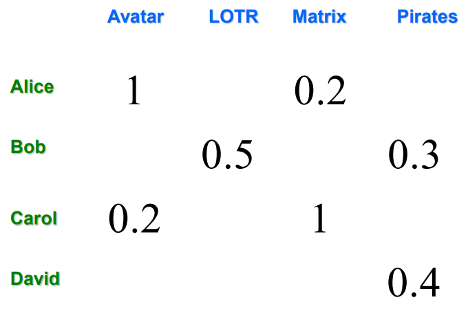
X: set of Customers
S: set of Items
R: set of Ratings
Utility function u: X x S -> R
 빈 칸들을 어떻게 채울 것인가
gathering known ratings for utility matrix
- explicit: ask people, 하지만 응답하지 않는 사람들이 많음
- implicit: learn from user actions(구매 이력, 클릭 유무, 검색 유무)
extrapolate unknown ratings from the known ones
Utility matrix is sparse
Cold start: 새로운 아이템이나 user는 rating 정보가 없음
Content based
user가 highly-rate한 item과 비슷한 item을 추천
- Item profile(set of features, vector)
Movies: author, title, actor
Text: set of important words(TF-IDF) - User Profile: weighted average of rated item profiles
-> cosine similarity로 user와 item 간 similarity 측정
장점: 다른 user data 필요 없음, 특이 취향 user에게 추천 가능, new&unpopular items 추천 가능, 설명 제공 가능
단점: feature를 찾는 게 어려움, 새로운 user에게 추천 어려움, overspecialization(user 취향 밖의 item은 추천 불가능)
Collaborative Filtering
유사한 rating을 매긴 user들의 set(N)을 고려하여 추천
- user-user CF(유사한 user 찾기): rating vector로 similarity 측정
Jaccard similarity(점수 고려 x) < cosine similarity(점수 고려 ↓) < Pearson correlation coefficient(점수 고려 o)
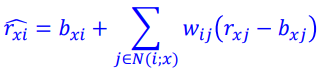
user들과의 similarity를 weight로 한 가중 평균으로 rating을 예측
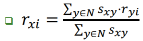
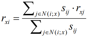
x: 예측 유저, y: 비슷한 유저, s: similarity - item-item CF(유사한 item 찾기): user 찾기와 같은 개념으로 구함
같은 metric으로 similarity를 구하고, 아래 식으로 가중 평균 rating 계산
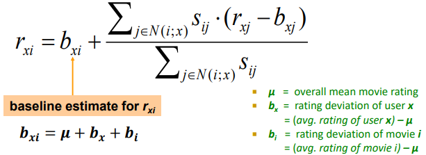
※ Baseline Predictor
사람마다 기준이 되는 점수가 다름(전체적으로 낮게 주는 사람, 높게 주는 사람..)
기준 점수의 차이 만큼을 보정해서 예측하도록 함
장점: 어떤 종류의 item이든 작동, 다른 사람들의 suggestion 사용 가능
단점: cold start, sparsity, popularity bias
■ Complexity: O(#customers)
-> pre-computation 필요: LSH, clustering, dimensionality reduction
■ Evaluation
RMSE, precision at top 10(error in top 10 highest predictions), rank(Spearman's) correlation
BellKor Recommender System
Global: 영화의 평균 평점에 baseline predictor 적용
Local neighborhood: 유저가 이와 비슷한 영화를 좋아하는 지를 적용
baseline prediction의 similarity 기반 weight average 식을 weight로 치환하여 ML 학습(SSE를 최소화하는 W 학습)
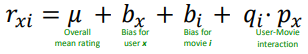
Latent factor based
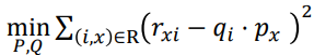
Utility Matrix를 Matrix Factorization으로 분해
(items과 users를 같은 dimension을 가진 각각의 matrix로 분해)
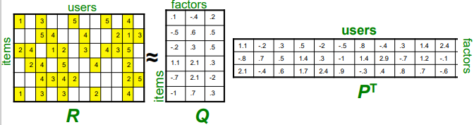 -> rating은 item matrix와 user matrix의 내적으로 표현됨
Utility Matrix에 값이 모두 차 있어야 SVD 적용 가능
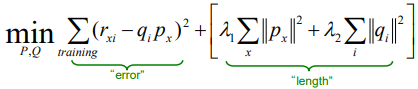
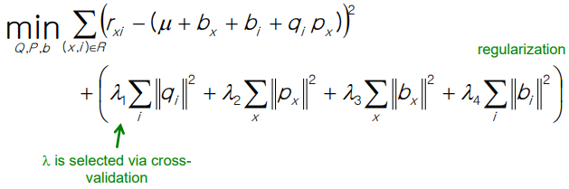
아래 loss 함수를 활용해서 gradient descent로 풀기
Regularization
overfitting을 막기 위해 regularization 도입
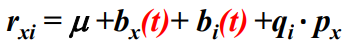
Bias Extension
user, movie 각각의 bias + user-movie interaction 고려
※ Temporal Bias: 특정 시간에 평균 평점이 모두 높아졌고, 오래된 영화일수록 더 높은 평점을 받는 경향이 존재
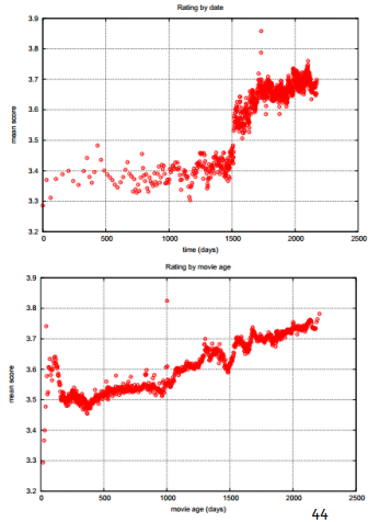
-> time dependence 추가
Deep Recommendation
Youtube Candidate Generation
input: 과거에 시청한 video embedding, 검색한 keyword token, 사는 지역, example age, 성별 등등
softmax: 수많은 동영상에 대한 확률(user vector와 내적이 클수록 높음)
LSH(nearest neighbor): 내적이 클 것 같은 동영상을 빠르게 고름
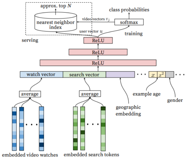
※ example age: upload된 지 얼마 안 된 동영상일 수록 클릭 확률이 높음 -> feature로 사용
Rating Prediction with additional information
item의 추가적인 정보(contents)가 있을 때 rating을 예측
item vector를 autoencoder로 생성(code vector)
- SDAE(Stacked Denoising Autoencoder)
noise를 가한 corrupted input을 본래 input으로 변환되도록 학습
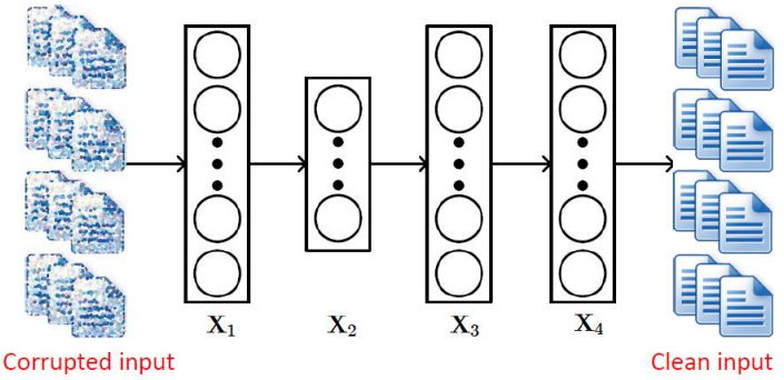
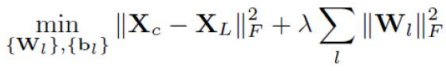
X_c: clean input, X_L: last layer(output)
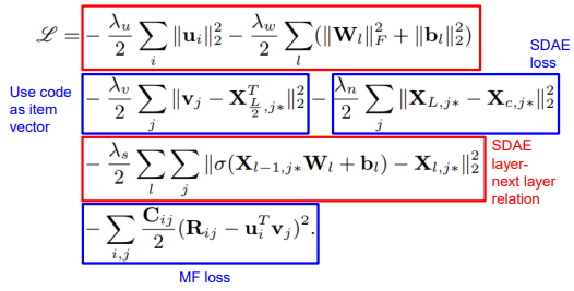
중간 layer(X_L/2)를 code vector로 사용해서 비슷한 content는 비슷한 item vector를 갖도록 함
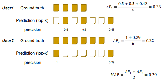
MAP(Mean Average Precision)
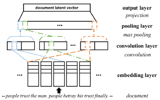
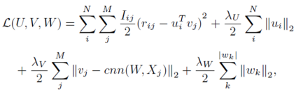
ConvMF
description document에서 주변 단어나 단어의 순서 등을 고려할 수 있도록 convolution 적용
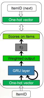
GRU4Rec
input: current item ID
hidden state: session representation
output: likelihood of being the next item
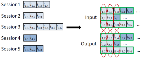
※ Session-parallel mini-batches
여러 세션을 하나의 mini-batch에 넣어서 학습
session의 길이도 다양하므로 여러 session을 이어 붙여서 사용
※ Negative sampling
모든 item에 대해서 softmax와 scoring을 계산하는 것은 너무 비효율적
-> one positive samples + several negative samples
negative sample은 mini-batch 안에서 뽑음
Loss functions
-
cross-entropy
-
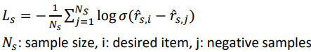
BPR(Bayesian Personalized Ranking)
-
Top1
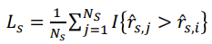 I: { } 안의 조건을 만족하면 1, 아니면 0
News Recommendation
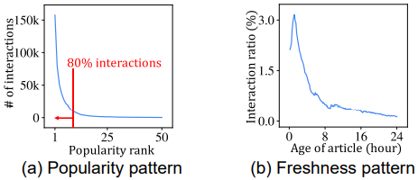
Popularity/Freshness pattern: 인기 있는 기사와 새로 나온 기사를 선호
PGT(News Recommendation Coalescing Personal and Global Temporal Preferences)
input: news watch history of user u, candidate news articles at time t, contents of news article
output: ranks of candidates for u, t
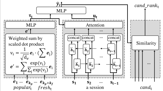
Global temporal preference: time t에 popular하고 fresh한 뉴스들을 하나의 vector로 요약
Personal preference: 시간 별로 u가 본 뉴스들(session)
Graph
Graph Representation Learning
각 node를 embedding하는 학습
node의 정보와 network 정보를 vector로 표현
-> anomaly detection, attribute prediction, clustering, link prediction, ...
어려움
size가 고정되어 있지 않고(구조가 복잡), node 간의 순서도 arbitrary함
DeepWalk
Random Walk Based Network Embedding
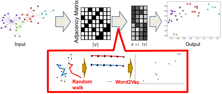
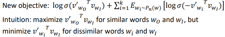
Random walk sequence를 sentence로 보고 word2vec 적용
Negative sampling을 통해서 가까운 node와 먼 node의 embedding이 다르게 되도록 학습
Node2Vec
network neighborhood끼리 feature space에서 가까이 위치하도록 embedding
neighborhood의 개념을 더 flexible하게 정의함
■ Objective function: 인접한 node의 내적이 크도록
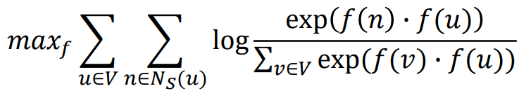
-> negative sampling을 통해 효율적으로 학습
Neighborhood 정하는 방법
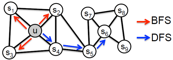
- BFS: Local microscopic view
- DFS: Global macroscopic view
Biased (2nd-order) Random Walks
1/p: 이전 노드로 돌아가는 가중치
1/q: outward node로 가는 가중치(DFS-like)
1: inward node로 가는 가중치(BFS-like)
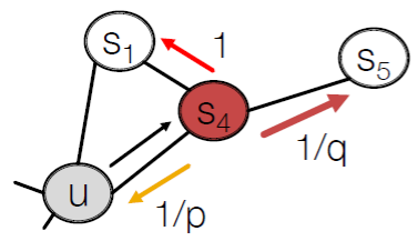
p, q를 semi-supervised로 학습
SIDE
signed directed network(negative edge가 있는)의 embedding 방법
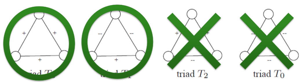
Theory of Structural Balance
친구의 친구는 친구다
적의 친구는 적이다
친구의 적은 적이다
적의 적은 친구다
Sign and Direction Aggregation
- Sign aggregation: structural balance 따름
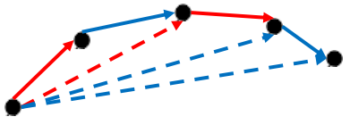
- Direction aggregation
Signed Proximity Term and Bias Term
- Signed Proximity Term: 내적으로 similarity를 표현
- Bias term: positive/negative edge가 많이 나가는/들어오는 node인지를 보정해줌(connectivity 표현)
Additional Optimization
- Delete one-degree node: one-degree node로 가게 되면 무조건 자신으로 돌아오게 되어있음 -> random walk 전에 삭제
-> training time 좋음 - Pass high-degree node: high-degree node만 너무 접근하게 돼서 오히려 less informative -> random walk에서 가급적 안 가도록
-> accuracy 좋음
※ Transductive vs Inductive
- Transductive: 모든 node(test node 포함)의 feature를 보고 training
- Inductive: 학습 시점에는 test node의 존재조차 모름, 훨씬 어려움
Graph Neural Networks(GNNs)
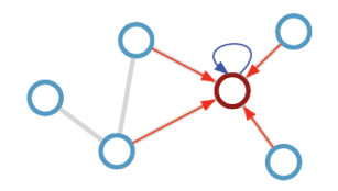
주변 node로부터 message를 받아서 합치는 과정
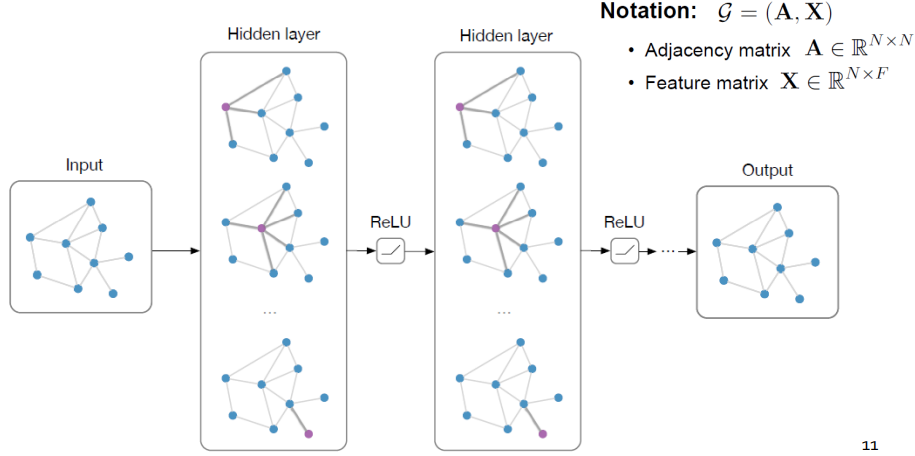
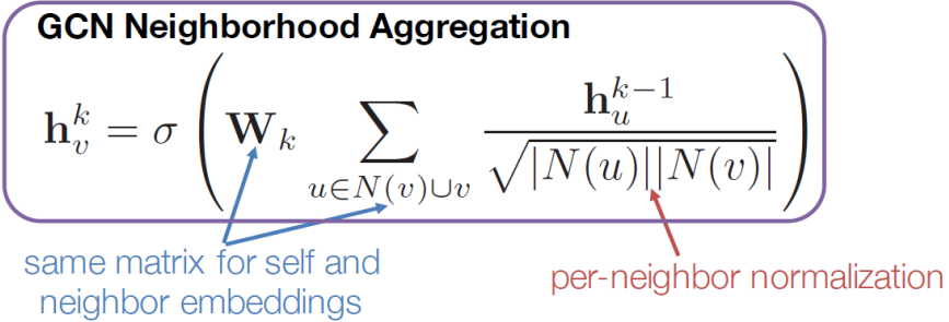
GCN(Graph Convolutional Network)
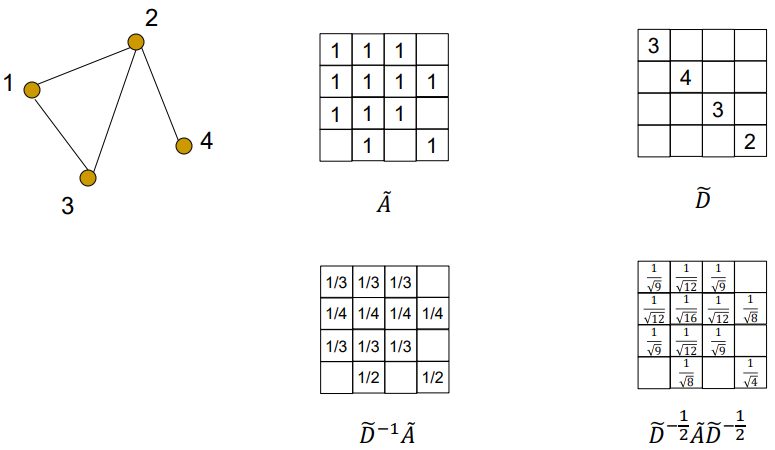
Citation Network
Citation 정보를 기반으로 논문 category 맞추는 문제

자기 자신도 참조하도록 A에 I를 더해줌
D(Degree Matrix): 이웃의 개수, D^-1/2: 역행렬에 루트
-> D^-1/2 A D-1/2: GCN의 per-neighbor normalization 효과
※ Oversmoothing: layer를 깊게 쌓다 보면 멀리 떨어져 있는 수많은 node의 정보를 평균 내기 때문에 node만의 특징이 사라지게 됨
real-world에서는 node 간 거리(hop)가 작음(평균 4 이하)
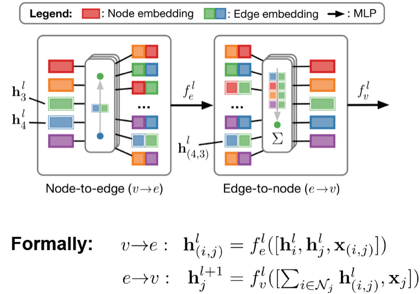
Edge Embeddings
edge 자체도 embedding할 수 있음
GraphSAGE
self embedding과 neighbor embedding을 concat(이전엔 그냥 더했었음)
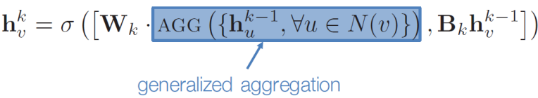
Aggregate function
- Mean: neighbor 수로 나눔
- Pool: element-wise mean/max
- LSTM: neighbor들을 random permutation 해서 LSTM에 넣음
GAT(Graph Attention Network)
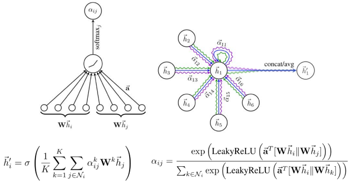
K: multi-head attention을 적용하여 변동성 줄임
Gated GNN
※ layer 많이 쌓았을 때 문제점
too many parameters, oversmoothing, vanishing gradient
GCN, GraphSAGE는 2~3 layer에서만 작동
-> Gated GNN
- parameter sharing across layers
- recurrent state update
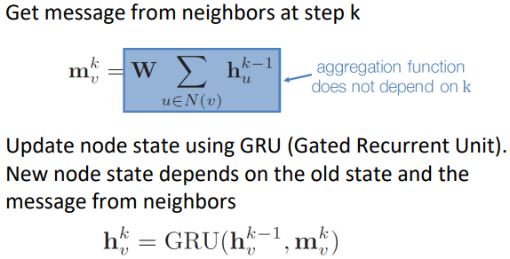
-> 20 layer 넘어도 작동
Time Series
Similarity Search
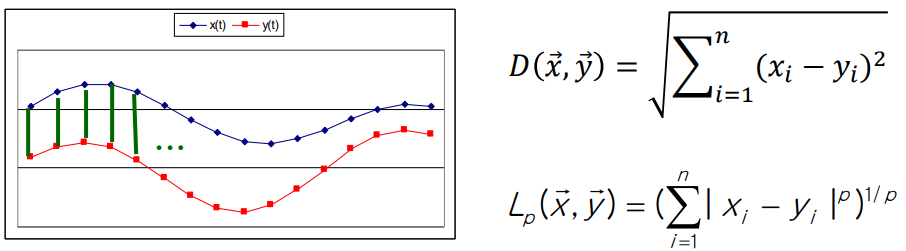
Distance Function
- Euclidean, Lp norms
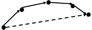
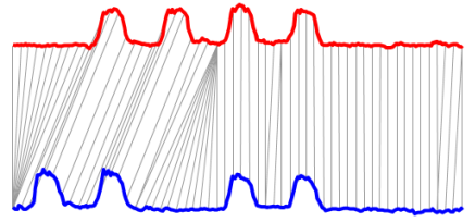
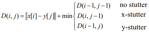
- Dynamic Time Warping(DTW)
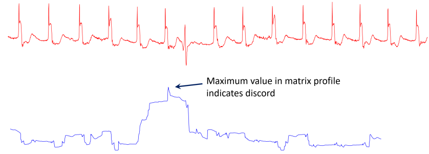
Matrix Profile
time series를 window로 나눔 -> 해당 시점에서의 window와 다른 모든 window와의 차이 중 가장 작은 값을 택하여 새로운 time series 구성
이렇게 구해진 profile로 abnormal detection, 반복되는 signal 찾기 가능
Linear Auto Regression
X: 시간에 따른 window input, y: X 다음 값, a: weight
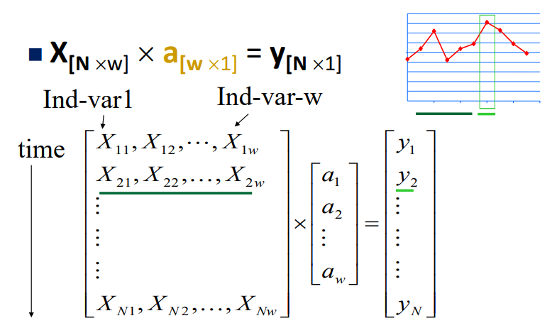
Least square fit으로 구할 수 있음
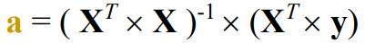
Moore-Penrose Pseudoinverse
Ax=y 방정식을 풀 때, A의 특성에 따라서 다른 A의 inverse를 곱하는 식으로 구함
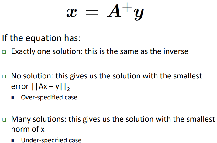
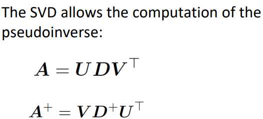
SVD로 구할 수 있음
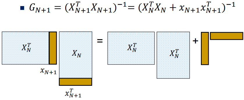
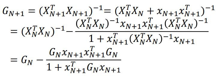
RLS(Recursive Least Square)
시간에 따라 X가 추가될 경우 빠르게 a를 업데이트하는 방법
Gain matrix를 recursive하게 업데이트해서 matrix inversion 없이 빠르게 새로운 a를 구할 수 있음
MLP 기반
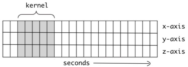
1-D CNN
시간축 방향으로만 stride
Multi-scale CNN(MCNN)
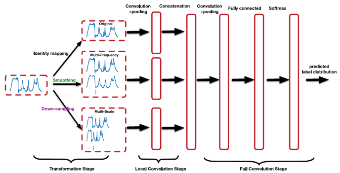
Multi-frequency: low-freq filter로 noise 제거(여러 개의 smoothing time series를 만드는 효과)
Multi-scale: long-term, short-term pattern 다양하게 잡아내도록