Linear Algebra - newlife-js/Wiki GitHub Wiki

By KAIST 주재걸 교수님

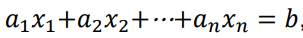
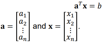
Linear Euqation:

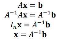
Inverse Matrix:

행렬 A에 곱해서 I(identity matrix)로 만드는 행렬(A^-1)

Linear System의 해를 구하는 데 사용
detA(ad-bc) = 0일 경우에는 Non-invertable(같은 직선 or 평행 직선이 존재하는 경우)

size(A) = m x n일 때,

m < n : variables > equations -> 무수히 많은 해(under-determined system)
m > n : variables < equations -> 해 없음(over-determined system)

Span:

벡터들의 모든 linear combinations의 set
(vector 2개로는 2차원을 구성, 3개로는 3차원을 구성할 수 있음, linearly independent할 때)
3번째 vector가 Span{v1, v2}에 속한다면, v3는 Span을 확장시키지 못함

b가 Span{a1, a2, a3}에 포함되어야 해가 존재
a1, a2, a3가 linearly independent해야 유일한 해가 존재

Subspace:

a subset of R^n closed under linear combination
subspace는 항상 Span으로 표현될 수 있음

Basis of a subspace(기저 벡터): a set of vectors that fully spans the given subspace H and linearly independent

basis는 unique하지 않음
basis의 vector수는 항상 같음(dimension)

Col Space(Col A):

행렬 A의 컬럼들에 의해 span된 subspace
rank A = dim Col A

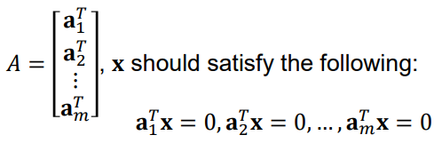
Null Space:

set of all solutions of a homogeneous linear system(Ax = 0)

Orthogonal Complement

Null space는 row space / col space와 다음과 같은 관계를 갖는다
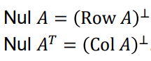
(Null space는 Ax = 0, 즉 A의 row들과 수직인 x의 집합을 뜻하기 때문)

Basis Theorem:

Any linearly independent set of exactly p elements in H is automatically a basis for H.
-> Any set of p elements of H that spans H is automatically a basis for H.

Linear Transformation

T(Transformation = function = mapping): x(input $\in$ Domain(정의역)) -> y(output = image $\in$ Range(치역) $\in$ Co-domain(공역))

T is linear if T(cu + dv) = cT(u) + dT(v)
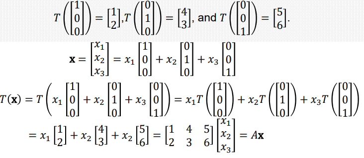
행렬곱[T(x) = Ax]을 통해 차원간 linear transformation 수행
A를 T의 standard matrix라고 함(A = [T(e1), T(e2), ..., T(en)])

at Neural Network

선형 변환 + 수축을 통해 비선형 classification을 수행할 수 있다.

출처: colah.github.io

Affine Layer:

bias가 더해진 linear Layer -> x에 값 1의 bias 차원을 넣어주어 linear layer로 변경해줄 수 있다.

onto(전사 함수):

range(치역)과 co-domain(공역)이 같은 경우, domain 갯수 >= co-domain 갯수
(Neural Network는 차원 변환이 대부분 일어나기 때문에 onto도 성립하기 어려움)

T maps R^n onto R^m if and only if the columns of A span R^m

col A = R^m

one-to-one(일대일 함수):

1 input이 1 output에만 mapping되는 경우, domain 갯수 = range 갯수
(Neural Network는 one-to-one이 안되도록 설계 / ex: 0 or 1로)

T is one-to-one if and only if the columns of A are linearly independent
참고

Least Squares:

over-determined system에서 최적의 해를 구하기 위해 사용하는 error term(b-Ax)
b-Ax를 최소화하는 최적의 해가 x_hat이고, b를 A subspace에 수선의 발로 내렸을 때 만나는 점이다.

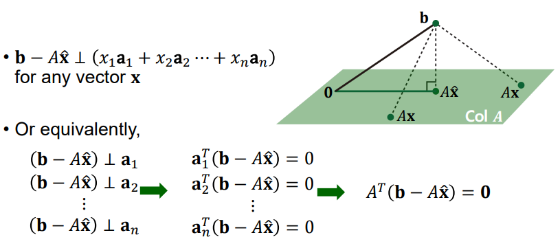
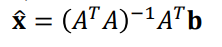
Normal Equation:

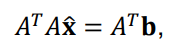
Orthogonal: 내적 = 0

Orthonormal: orthogonal하면서 길이가 1

Gram-Schmidt Orthogonalization:

linearly independent basis -> orthogonal basis로 변환

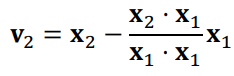
x2를 x1에 orthogonal projection하여 수선의 발에서 x2로 가는 수선 벡터를 v2로
x3를 Span{v1, v2}에 projection하여 수선의 발에서 x3로 가는 수선 벡터를 v3로
...
v_n = x_n - proj_Wn-1(x_n)

QR Factorization(행렬 분해)

A = QR

Q(m x n): orthonormal basis for Col A(m x n)
R(n x n): upper triangular invertible matrix with positive entries on diagonal

a1 = u1 * ||v1||
a2 = k1u2 + k2u1(k1 = ||v2||, k2 = x2 u1 내적)
...
a_n = j1u_n + j2u_n-1 + ... + j_n-1*u1 (j1 = ||v_n||, j2 = x_n u_n-1 내적)
(u1~u_n-1: Q의 원소, ||v1||/k/j: R의 원소)

--> upper triangular matrix R이 만들어짐

Eigenvector

Ax = λx를 만족하는 nonzero vector x(λ를 eigenvalue라고 함)
(A-λI)x = 0

Eigenspace: (A-λI)x의 Null space

det(A-λI) = 0(characteristic equation)의 해 λ를 구하면 됨
Algebraic multiplicity: Eigenvalue가 몇중근인지를 말함, multiplicity 이하의 eigenspace dimension을 갖는다

Diagonalization

D = P^-1AP
P의 각 컬럼은 A의 eigenvector이면서, D의 각 원소는 eigenvalue이어야 함
P의 역행렬이 존재하기 위해서는 정사각 행렬이면서 각 컬럼들이 linearly independent해야 함

EigenDecomposition(of A) : A = PDP^-1

y = P^-1x: change of basis(y는 x의 새로운 eigenspace에서의 좌표값)
z = Dy: Element-wise Scaling
T(x) = Pz: back to original basis

퀴즈

Singular Value Decomposition(SVD)

U, V는 orthonormal basis matrix
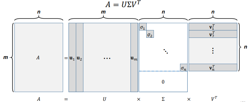
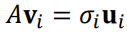
AV=U∑
->

※ symmetric matrix는 orthogonally diagonalizable(n개의 orthogonal한 eigenvector를 가진다)
Spectral Theorem: symmetric matrix는 n개의 real eigenvalue를 갖고(허근이 없음), 각 eigenvalue는 multiplicity 만큼의 차원을 갖는 eigenspace를 갖는다. 각각의 eigenspace는 서로 orthogonal하다.
-> orthogonally diagonalizable하다..

Spectral Decomposition:

Eigendecomposition of symmetric matrix(S = UDU^T)
-> orthonormal 성분별로 eigenvalue만큼 가중치를 곱해서 더한 형태

Positive Definite:

Semi-positive definite:

ex) AA^T
x^T AA^T x = (x^T A)(A^T x) = ||A^T x||^2 >= 0

모든 직사각 행렬에 대해 SVD는 항상 존재
eigendecomposition이 불가능한 정사각 행렬에 대해서도 SVD는 존재
symmetric positive definite matrix에 대해서는 SVD = eigendecomposition

Low-rank approximation:

A와 가장 비슷한 형태를 띄는 Rank r의 행렬 A_r을 찾는 것(argmin||A-A_r||_F)
∑의 σ는 all positive로 함(eigenvector의 방향만 반대로 바꿔주면 되므로)
σ는 내림차순으로 배치(eigenvector의 순서 바꿔줌)하여 r개만 남김
SVD의 U 매트릭스의 r개 컬럼만 가져오는 것

PCA(Principal Component Analysis)

Orthogonal projection을 통해 Dimension reduction을 수행
coordinate system을 변화시켜서 적은 수의 principal components만으로도 data 분포(분산)를 잘 설명하도록 하는 것

Zero-centering(mean substraction)
Covariance 계산(Cov(X) = 1/(m-1)*X^TX: symmetric)
Covariance Matrix의 eigenvector들이 principal component들이 된다.
Covariance는 유지하면서 orthogonal한 vector들(U)을 구하고, σ를 내림차순으로 정렬하여, 상위 n개만 뽑아 dimension reduction을 한다.
Cov(X)의 eigendecomposition = 1/(m-1)*Uσ^2V^T 를 구하는 것은
X의 svd = UσV^T 를 구하는 것과 같다.
※ explanation ratio: σ n개의 제곱합 / σ 전체의 제곱합