by 서울대학교 문태섭 교수님

Supervised learning의 한계

• requires LARGE training data in BATCH
  하지만 현실에서는 데이터의 특성(분포)이 계속 변함, target task도 계속 많아지고 어려워지지만 학습 데이터는 적음
  
• DL models are EXTREMELY complex
  모델들이 critical decisions(의학 진단, 자율 주행)을 내리는 경우가 많아 설명할 수 있는 게 중요함
  unfair bias를 갖게 되는 경우도 많음

Adaptive Machine Learning(AML)

Related Problems

• Multi Task Learning
  다양한 task에 대해서 한 번에 학습(새로운 task에 대해서는 no)
  
• Transfer Learning
  새로운 task에 대해 학습(overcome forgetting에 대해서는 no, only forward transfer)
  
• Domain Adaptation
  

Continual(Lifelong) Learning

Multi-task & Sequential learning
새로운 테스트 데이터(good forward transfer)와 이전 데이터(overcome catastrophic forgetting) 모두 잘 처리해야 함

• Task-incremental learning(Task-IL): 어떤 task인지 주어졌을 때 0/1 판별
• Domain-incremental learning(Domain-IL): 어떤 task인지 주어지지 않고 0/1 중에 하나만 고르도록
• Class-incremental learning(Class-IL): 모든 task에 속하는 class(0~9) 판별
  

Plasticity-Stability Dilemma

• Plasticity(forward transfer): 새로운 task를 학습하기 위해 parameter가 잘 변경되어야(plastic) 함
• Stability(overcome catastrophic forgetting): fine-tuning이 이전 데이터에 대해서도 잘 작동(not forget)해야 함

Additional requirements

• scalable(task 종류가 많아질 수 있음)
• positive backward transfer(이미 학습한 task가 들어왔을 때 더 빠르게 학습)
• learn without task label(task boundary가 주어지지 않은 경우에도 잘 작동)

Common approach

• Regularization: identify important weights for each task
• Parameter isolation: expand the network for a new task
• Memory replay: store and generate past task data

Regularization-based

Identify which nodes/weights are important for each task
Put high regularization to the important nodes/weights
Mainly focus on the stability

Elastic Weight Consolidation(EWC)

• single task case
  
  p(θ|D) = p(D|θ)P(θ) / p(D), p(D)는 control할 수 없음..
  -> two tasks
  task1 학습하고 난 정보를 prior로(regularizer로) 사용
  

■ Laplace Approximation
p(θ|D)을 Gaussian distribution으로 근사(최빈값을 mean으로, covariance는 Fisher Information Matrix로 구함)

※ Synaptic Intelligence(SI)

Variational Continual Learning(VCL)

EWC처럼 θ의 point estimate를 구하는 것이 아니라, θ의 distribution(q_t)을 구함

Use a tractable distibution q_t(θ) to approximate p(θ|D_1:t)
Maximize ELBO(Evidence Lower Bound)

Adaptive Group Sparsity based CL(AGS-CL)

Node-based importance measure & regularization
Node-level regularizations based on group sparse norms
node-level이기 때문에 weight-level보다 적은 regularization parameters만 사용

Replay Memory-based

Gradient episodic memory(GEM)

task당 적은 수의 sample들을 메모리(M)에 저장


g^˜: 새로 들어온 task 데이터에서의 gradient / g_k: 이전 task 데이터에서의 gradient -> 내적이 0보다 크도록(방향이 비슷하도록)

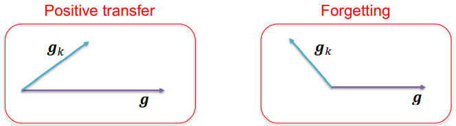
※ GEM은 연산과 메모리 cost가 큼

Averaged GEM(A-GEM)

지나간 task들의 평균 episodic memory loss를 constraint로 사용

-> GEM보다 훨씬 좋은 연산/메모리 efficiency

※ (A-)GEM은 데이터 자체가 아니라 데이터의 loss의 gradient를 사용하기 때문에 actual data의 정보를 저장하는 효용이 떨어짐

Experience Replay(ER)

Directly train on the examples stored in a memory
새로운 데이터 batch(g)만큼을 memory로부터 batch(g_ref)를 뽑아서(doubled minibatch) gradient를 구해서 parameter update

Parameter Isolation-based

regularization, memory-based는 fixed model capacity(memory size)만을 고려
새로운 task에는 추가적인 neural resources를 할당

Progressive Neural Networks(PNN)

기존의 NN(column)은 freeze하고, 새로운 NN을 확장하여 과거 column으로부터 hidden activation을 받음

※ task가 커지면 model도 너무 커짐

Dynamically Expandable Networks(DEN)

필요할 때만 NN을 확장(selectively utilize prior knowledge)
기존의 NN으로 새로운 task에 대해 학습을 해보고,
loss가 기준 이상 크면 node를 추가한 후 다시 학습
이전 step에서의 파라미터와 비슷한 지를 확인해서 split&duplicate 과정도 거침

Piggyback

task별로 다른 binary mask를 학습해서 task마다 적용하도록

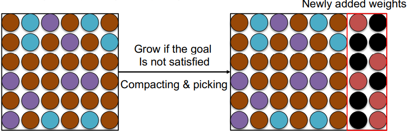
Compacting, Picking and Growing(CPG)

DEN과 Piggyback을 합침

• compacting: model을 압축
  
• picking: 새로운 task에 대해서 binary mask를 학습
  새로운 task에 필요한 parameter는 기존 parameter에서 masking된 부분에 채워 넣고, 공통으로 사용할 parameter는 같이 사용
  
• growing: 필요할 때 model capacity를 늘림
  

Meta Learning

새로운 task가 들어왔을 때 적은 데이터로도 빠르게 학습할 수 있도록

여러 task들 간에 shared structure(유사성)가 있다고 가정

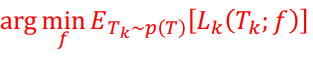
p(T): Task들의 distribution

■ 문제 정의: 적은 training samples로부터 test samples를 예측
예) Few-shot classification
여러 task에 대한 training/test dataset을 포함하는 Meta-training dataset이 존재

Model-based

task distribution에 대해 loss function이 가장 작아지는 model(f)을 구하는 것

Memory-Augmented Neural Networks(MANN)

Omniglot 데이터셋 사용(5-way, 10-shot -> episode당 50 samples)

Neural Turing Machine(NTM)

Memory에 저장된 값들과 controller key의 cosine similarity softmax 확률을 weight로 사용하여 read
가장 적게 쓰이는(LRUA) 메모리 위치에 업데이트


controller로는 LSTM을 사용하여 set이 아닌 연속된 데이터를 input으로 받음
x에 대한 label(y)은 1씩 offset으로 시간차를 주고 input으로 넣어줌(정답인지 아닌지를 다음 LSTM cell에서 정보를 저장)

Simple Neural Attentive Meta-Learner(SNAIL)

Conditional Neural Processes(CNP)

MANN과 SNAIL은 input을 sequence로 받기 때문에 input의 순서가 영향을 미침
-> set 형태로 input을 줌

embedding function과 classifier를 학습

Optimization-based

pre-trained model에 fine-tuning을 해서 adaptation하는 방법

Model-Agnostic Meta-Learning(MAML)

few shot만으로도 initial θ를 찾을 수 있도록 여러 task의 파라미터로 gradient descent update를 해 줌
initial θ를 잘 찾아 놓으면 adaptation이 쉬워짐

※ First Order MAML(FOMAML): backward pass의 Hessian matrix를 0으로 해서 연산을 간편화해 근사

Metric-based

second-order optimization 없이 학습하기 위해 non-parameteric learners를 사용
meta-test에서는 K-NN과 같은 non-parameteric method를 사용 / meta-train에서는 parameteric method 사용

Matching Networks

Prototypical Njetworks

Euclian distance로 prototype과 test data의 차이를 계산