Return to TOC

The first view you see when MuhRec starts is the place where you can enter information about the projection data (Figure \ref{fig_ProjectionGeometry}). The upper part of the view is used to specify paths and filenames. The lower part describes the projection geometry.

The projection data (radiographs) is the input to the reconstruction and in contrast to most other reconstruction tools you never have to explicitly build sinogram files. You can also provide open beam and dark current reference images in this view. The projection files are chosen using the browse button. Locate and select any projection file in the data set. When you return from the file dialog the filename mask appears in the path field. When you enter the file mask of the projection files manually the general format is basename####.ext, where the base name can be any string. The file extension is used to determine image file type and must be correctly specified (currently supported are fits extensions fits,fit,fts and TIFF extensions tif and tiff). Finally the # are place holders for the file index. The number of place holders defines how the zero padding should be used. Some examples using two place holders: proj_##.tif will give the filenames proj_00.tif to proj_99.tif, and thereafter proj_100.tif etc. If you omit the # at all the indices will be inserted after the base name and before the extension without zero padding.

Once you have defined projection path you have to set the first and last projection indices as well as the file stride. The stride can be used to reduce the number of projections for test purposes when you want a quick reconstruction. The first index can be any positive number smaller than the last projection index.

During the experiments it may happen that projections are retaken. Depending on the acquisition system these files may remain in the sequence. MuhRec provides a skip list to exclude retakes from the reconstruction. A dialog is povided to make the search for the retakes easier. The dialog use the intensity variations in the dose ROI and you only have to give the expected number of projections and the dialog finds the indices with the lowest dose. The skip list created when you reduce the number of expected projections. A word of caution; the plot is instantaneously updated so when you retype the number it redraws the plot for each digit with the effect that the first digit tries to add all projections to the skip list. The better way is to decrease step wise using the decrease button of the field.

Below the projection information you find some fields for rotation, flip. The projection flip works well, but there are some problems with the rotation.

The reference files are entered in the same manner as the projections. Both open beam and dark current images are required to located in the same directory. You also have to set the first reference image index and the number of references. These numbers are set for both open beam and dark current image separately. If you don't have any reference images just set the number of references to 0. By pressing the button to the left of the field, you can save some time locating the path of the reference data. This will copy the projection file name to the reference field.

When all file parameters are set you can click the preview button to see the projection in the display area to the right. There is also a slider that lets you browse through the projection data. Which can be handy when you search for the geometric extents of the projection data.

Finally, you can also set the pixel size of the projections (unit mm). This information is needed if you want the gray-levels of the pixels to have the unit cm^-1. The pixel size is also written as resolution in the slice image files.

Once you have selected the projection data, you need to the define the geometry of the reconstruction. This includes defining region of interest that inscribes the sample on all projections and to select which slices you want to reconstruct. A narrow choice reduces the amount of data that need to be processed. The most important is the center of rotation which has to be determined to sub-pixel accuracy. Other parameters defines the number of slices and the margins of the projections. The projection configuration dialog helps you to find the center of rotation. The estimated value should be seen as a starting point for the fine tuning. Depending on the sample shape, noise level, and artifacts the estimate may deviate by several pixels from the true center. If your projection data was acquired with a tilted axis of rotation it will have an impact on the reconstructed data. For small tilts, this looks like a shift in center of rotation. Only the slice you tuned the center of rotation for will be correctly reconstructed, on other slices the degradation will increase with the distance from the tuned slice. Small tilts (<1°) can be corrected. The correction for larger tilt angles is still a pending feature.

The amount of memory required for the reconstruction is estimated to give you an idea if the task is feasible for your computer. You can control the memory usage by changing the geometry of the reconstructed image, i.e. change the margins or number of slices. In the interactive mode MuhRec3 is keeping all projection data and the reconstructed volume in memory. When the total size exceeds the available memory, MuhRec offers you the option to stream directly to disk. Then the slices will the stored on the location specified on the results view.

The region of interest is marked in the projection preview image. The region used for dose computation is also marked in this display.

Once you have set all parameters it is recommended to save the parameters. You save the parameters by selecting save or save as in the file menu. Alternatively, you can also press CTRL-S which performs the same action. In a way the parameter file is a documentation of your reconstruction. It also allows you to load the parameters at later moment if you would like to do adjustments or reconstruct a new part of the samples. You can also use the parameter file for command line reconstructions and batch processing. For more details about the command line mode please read this section. The saved parameters can be loaded into the GUI by using the File-Open menu.

The current reconstruction configuration is stored in the file CurrentRecon.xml every time you start a reconstruction. This file is stored in the folder .imagingtools in your home directory. This file will automatically be loaded when you start Muhrec next time. When you install a new version of MuhRec, it can make sense rename the CurrentRecon.xml as the new version may new new parameters. You can remove CurrentRecon.xml if you have starting problems caused by a corrupt configuration. This can even be done in muhrec by selecting the menu Options=>Remove CurrentRecon.xml.

When the geometry is configured you can switch to the processing tab, On this tab, you can configure a chain of preprocessing operations (modules) to apply on the projection data prior to reconstructing. Some modules are a natural part of the reconstruction (e.g. Normalisation and Projection filter), while others are added to suppress unwanted information. This means you can add new modules if your data requires some special treatment and you can edit the module parameters manually in the field to the left of the module list or by wizards. Most modules have a wizard to help with the configuration through visual feedback showing the effect of each operation. It may take some time to open the wizard for the modules. This delay is because the data is read and processed by the modules that precede the selected module.

New modules are added by pressing the add button. The dialog that opens lets you select a library containing modules (StdPreproc is chosen by default). The combo box lets you select a module. Confirm you choice by pressing OK. The new module can be dragged to the intended position in the processing chain.

It is also possible to change back-projector and configure its parameters. Mostly it is sufficient to select a back projector and use the default parameters. Changing back-projector parameters is an advanced topic that requires understanding of the implementation of the algorithm. The most important parameter is the buffer size. This parameter has a direct effect on the memory consumption during the reconstruction.

Once the parameters for the reconstruction have been set, you can start the reconstruction by selecting the reconstruction menu. There are two modes to consider; for small data sets you can do the reconstruction in interactive mode. This means that you can adjust the gray levels and select destination folder, file name, and file format after the finished reconstruction. When the selected matrix is too large for the available memory a dialog that gives you the options to reconstruct directly to disk using the configuration on the matrix tab or to cancel the started reconstruction.

If you select the direct streaming option for the reconstruction there will be no output in the slice display.

It is often recommended to make a small test reconstruction to check the quality of the selected parameters. Select between 16 and 64 slices in a relevant region of the sample and start reconstruction. It may take some iterations until you have tuned everything as you want it.

• Center of rotation
• Axis tilt
• Artefact cleaning

This may take some time and in the beginning it is recommended to deactivate the cleaning modules to speed up things. When you are satisfied with the result you can reconstruct the whole data set in a single run.

When the reconstructor finished processing the data you are automatically directed to the 'Results'-tab.

Here, you see a histogram of the reconstructed data. The vertical lines in the histogram show the gray-level interval used to display the reconstructed slice in the viewer. These levels will also be used to in the conversion to integer formats. You can change the gray level interval in the entry fields on the top. Two convenience buttons are provided to select intervals based on 95% and 99% of the pixels.

A slider can be used to browse through the slices. By sliding through the slices you can inspect the slices to check that the gray interval is correctly set. You can also check if there are any artefacts that needs attention in your data.

Once you are satisfied with the image settings and reconstruction quality you can save the slices. To do this you have to select the destination folder and enter the file mask for the slices. The mask has the same format as the projection data i.e. base####.ext. The extension must be entered manually as it is not adapted to the selected file type. The last selection to make is the file format which can be tiff with different bit depths.

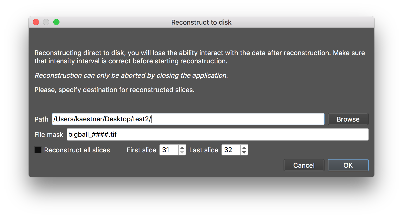
When you do the final reconstruction it is likely that you have to stream direct to disk and lose the interaction feature. The same dialog as reconstruct to disk appears asking for the destination will appear if this is needed. The memory size limit can be set in the parameter file.

It is possible to store the current configuration in the geometry list using the application menu item Geometry. This can be used to test the effect of different settings without losing the original settings. Each parameter set will be stored with the central slice to make comparison easier. If you have reconstructed several slices on different places you can use the entries of the list to calculate the axis tilt.

Cone beam reconstruction requires a different back-projection module and an extended geometry compared to the parallel beam reconstruction previously described. The typical use case is for X-ray data, but it is also beneficial to use conebeam reconstruction for neutron imaging data. This corrects for the penumbra blurring that can be observed for low collimated beams when large samples are scanned.

Starting from a clean configuration [File]=>[New] you have to make some changes that are described below.

Cone beam reconstruction is a feature under development. This means you cannot expect the same reconstruction speed as you are used to with the parallel beam back projection. In fact, you may have to wait longer time for a few slices depending on system.

The cone beam reconstruction code was derived from the open source implementation of the FDK algorithm developed in plastimatch (https://www.plastimatch.org/) and adapted to work in the MuhRec framework.

The geometry needs to be described with more detail for cone beam reconstruction. This is enabled by setting the check box Cone beam in the geometry field of configure projections. This activates the "Advanced geometry" tab. In this tab, you can set the distances from source to the rotation axis of the object/sample and to the detector. These distances define the magnification for the measurement and should be available from the experiment meta data. The next parameters to set is the position where the beam hits the detector perpendicular to the detector plane (piercing point). This position is given in pixels relative to the global detector area.

The typical preprocessing chain for a cone beam reconstruction includes

• Projection normalization and negative logarithm
• Spot cleaning.
• Ring cleaning.

The projection filter used for parallel beam reconstruction is not needed as it is part of the CBCT back-projection module. Finally, you also have to change the back-projection module which is located in the library file libFDKBackProjectors. It is recommended to use the fdkbp_single module as this module process the data faster (with a negligible loss of quality).

Return to TOC