KipTool manual: AdvancedFilterModules - neutronimaging/imagingsuite GitHub Wiki
Return to Image Processing modules
The AdvancedFilterModules implement an advanced filter for edge-preserving smoothing. From the Image processing tab click the Add button and select the AdvancedFilterModules libraries, the following modules are available:
The Inverse Scale Space Filter is an edge-preserving de-noising filter based on the paper by Burger et al. 2006. The filter solves the differential equation:
where f is the original image, u is the image solution and v is the image solution at the previous step, and
are regularization parameters.
An iterative solver is used on the discrete equations. Here the total solution time can be selected using a number of iterations,
, and time increments,
. It is important that the value of
is less than 0.125 to maintain numerical stability of the solution. Decrease
if you want to improve the quality of the solution but then
must be increased to maintain a constant
. The sensitivity to noise is decreased for small
. Another constraint is that
otherwise the eigenvalues of the system become complex and the solution will oscillate. The equation works best when the data is normalized to zero-mean and variance equal to one, this can be done automatically by setting the parameter autoscale to true. This setting will compute a new normalization for every data set, i.e. if you tune the filter for a small ROI and change to the full image a new normalization will be made and the settings used for the sub-image are not guaranteed to be perfect for the full view image.
The error curve shows how the filter performs. The figure below shows an error plot for the ISS filter when it runs to stability. Here, it can be seen that after a large change the filter brings the error back to a minimum, i.e. the original image is obtained again. Ideally, you should never let the filter run beyond the error curve peak and mostly the best result is obtained in the interval which is marked in the plot. You can also use the error curve to check if the filter settings are stable. A stable filter produces a smooth error curve while the in-stable solution produces an oscillating error curve.

Figure: An error curve from the ISS iterations.
A quality check is to inspect the difference image. A well tuned ISS filter should only show noise and artifact in the difference image between the original and filtered. If you see any structures you know that the filter is modifying the structures in the image. This is an indication that you should try to tweak the parameters a bit more.

Figure: An image before and after ISS filtering and their difference.
For tuning, we recommend using a small ROI eg. 100x100x20. The chosen region should not contain too great contrast variations. In our experience, it is best to try using the default parameters as a starting point for filter tuning and observe the error curve. A great for the solution time could be set to identify the
and with that find a good
for your filtering task. Next step is to refine the values of
and
. This is done iteratively using a sequence like
| Iteration | ||
|---|---|---|
| 0 | 1.0 | 0.25 |
| 1 | 1.0 | 0.1 |
| 2 | 0.5 | 0.1 |
| 3 | 0.5 | 0.05 |
| 4 | 0.25 | 0.05 |
For each iteration, you should check
- Image improvement
- Difference between original and filtered. Can you see image structures in the difference image? If structures are visible you should continue tune the filter.
- Changes in the histogram. Do you get a significant improvement in peak widths? This indicates a successful improvement in SNR.
At some point, you will lose relevant image features. So you'll have to pay attention to this.
The ISS filter module also provides further parameters for experimental purposes. These are the regularization that can be chosen between the ROF model and a TV-1 model (also in Burger et al. 2006). We have little experience with the TV-1 model, but so far we prefer the ROF which is set as default. The other parameter is the choice of the initial image for the processing. Our experience is that the original image produces more reliable results with the current implementation of the filter.
If you are interested in seeing the progress of the filter there is a switch to save the middle XY-slice for each iteration. This can be useful for demonstration and debugging purposes.
The diffusion filter module implements a filter based on the Perona and Malik 1990 using regularization according to Catte et al. 1992 and the AOS scheme introduced by Weickert et al. 1998.
Where the diffusivity function
is a treshold function applied to the Laplacian of the image smoothed by a Gaussian filter with the width . The threshold,
, controls the filter behaviour at edges in the image such that edges have low diffusion, i.e. blocking the filter operation, while flat regions have diffusion approaching one and thus experience the full diffusion effect. In all, this results in the edge preserving smoothing properties on the filter.
The diffusion filter is controlled by four parameters:
-
- Diffusivity smoothing.
-
- Diffusivity threshold.
-
- Solution time increment.
-
- Number of iterations. The default parameters are usually a good starting point for data with zero mean and std dev = 1.
The smoothing reduces the impact of noise in the Laplacian as is shown in the figure below. A noisy diffusivity map would not be able to reduce the noise very well as the steep outliers of the noise also would be protected from smoothing.

Figure: Using Gaussian smoothing of the Laplacian improves the diffusivity map.
The values in the diffusivity map are calculated using the diffusivity function above. The value of is best found using the cumulative histogram of the Laplacian image. Usually, images have far fewer edge pixels than 'bulk' pixels. therefore the threshold is set to start reducing the diffusivity for a few percents of the Laplacian pixels that are obvious outliers in the data. The green curve in the figure below will produce a good filter effect while the orange one will allow smoothing for most pixels including the edges we want to preserve.

Figure: The threshold level () is chosen with the help of the cumulative histogram of the smooth Laplacian.
The next figure demonstrates how the Laplacian smoothing focusses the blocking regions to the real edges in the image and reduces the number of spurious edges. There is, however, a risk that the smoothing may cancel low contrast edges, which then are left unprotected from the diffusion process.

Figure: Diffusivity maps for different smoothing strength applied to the Laplacian of u.
Note: the Laplacian image and the cumulative histogram will be implemented in the tuning dialog in a future version of KipTool, see issue 304 .
The diffusion filter is an iterative filter that requires some iterations to achieve the desired filter effect. The total solution time is defined as . The computing time is proportional to the number of iterations,
, and the accuracy and filter stability depends on the time increments
. Solutions with small increments are usually less sensitive to noise.
A quality check is to inspect the difference image. A well-tuned diffusion filter should only show noise and artifact in the difference image between the original and filtered. If you see any structures you know that the filter is modifying the structures in the image. This is an indication that you should try to tweak the parameters a bit more.
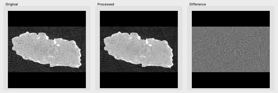
Figure: An image before and after ISS filtering and their difference.