Project 3 - ncbi/workshop-asm-ngs-2022 GitHub Wiki
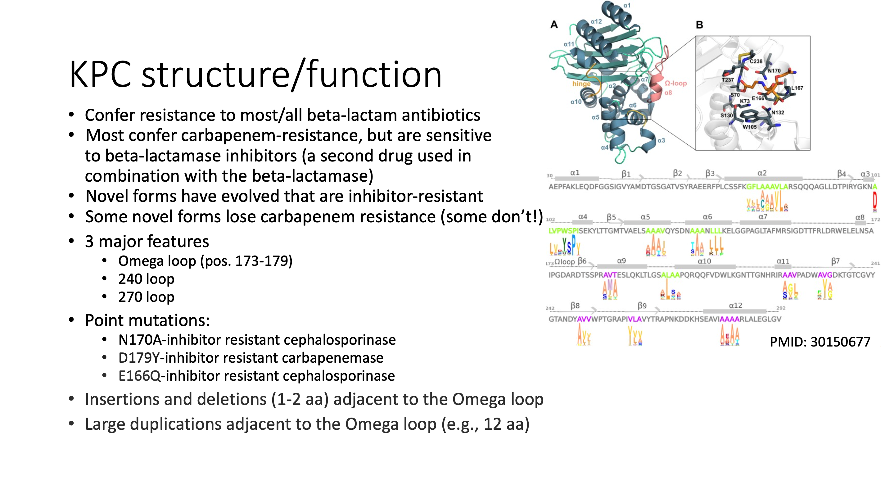
BlaKPC is an important resistance gene to carbapenemases which are a family of beta-lactamases that are usually used as the last-line of defense to highly resistant organisms. The most common blaKPC allele is blaKPC-2, which is a 293 amino acid protein that we find in about 17,000 isolates in the Pathogen Detection system. Insertions near the Omega loop are known to affect substrate binding and phenotype, but to our knowledge publications have not come out investigating positive selection on amino-acid substitutions in blaKPC. Here we look at all the 293-aa blaKPC genes in MicroBIGG-E to see if we can find sites under positive selection in this enzyme.
Why only 293-aa blaKPC sequences? Basically to make the project simpler. If we were doing this for a paper we might include all blaKPC sequences, or even add in other closely related class-A carbapenemases. But these genes are under heavy selection and some include things like tandem duplications that tend to confuse multiple sequence aligners. So to do this right with all the sequences you would need to manually edit the alignment, keep track of coordinates and deal with other complexities that we don't have time to go into here.
mkdir -p ~/project3
cd ~/project3Here we use the google command-line interface for BigQuery,
bq to run a
query and get the output into a text file. Note: You may get an error
message about some configuration that needs to be done. Just run the bq command
a second time and it should work.
bq query --use_legacy_sql=false --max_rows 50000 '
SELECT contig_acc, contig_url, start_on_contig, end_on_contig, strand, element_symbol
FROM `ncbi-pathogen-detect.pdbrowser.microbigge`
WHERE element_symbol LIKE "blaKPC%"
AND element_length = 293
AND amr_method IN ("EXACTX", "EXACTP", "ALLELEX", "ALLELEP", "BLASTX", "BLASTP")
' > 293aa_kpc_contigs.out
Lets take a look at the results
head 293aa_kpc_contigs.out+----------------------+----------------------------------------------------------------------------------------------+-----------------+---------------+--------+----------------+
| contig_acc | contig_url | start_on_contig | end_on_contig | strand | element_symbol |
+----------------------+----------------------------------------------------------------------------------------------+-----------------+---------------+--------+----------------+
| DAGJCA010000251.1 | gs://ncbi-pathogen-assemblies/Klebsiella/858/709/DAGJCA010000251.1.fna.gz | 152 | 1033 | + | blaKPC |
| DAGFMJ010000187.1 | gs://ncbi-pathogen-assemblies/Klebsiella/874/735/DAGFMJ010000187.1.fna.gz | 308 | 1189 | + | blaKPC |
| DAGAHK010000102.1 | gs://ncbi-pathogen-assemblies/Klebsiella/1019/705/DAGAHK010000102.1.fna.gz | 10658 | 11539 | + | blaKPC |
| DAFWJT010000348.1 | gs://ncbi-pathogen-assemblies/Klebsiella/1141/057/DAFWJT010000348.1.fna.gz | 165 | 1046 | + | blaKPC |
| DAJACB010000057.1 | gs://ncbi-pathogen-assemblies/Escherichia_coli_Shigella/1386/299/DAJACB010000057.1.fna.gz | 7204 | 8085 | + | blaKPC-3 |
| NZ_KL407350.1 | gs://ncbi-pathogen-assemblies/Klebsiella/33/733/NZ_KL407350.1.fna.gz | 26561 | 27442 | + | blaKPC-3 |
| NZ_LAKK01000012.1 | gs://ncbi-pathogen-assemblies/Klebsiella/66/427/NZ_LAKK01000012.1.fna.gz | 3087593 | 3088474 | + | blaKPC-3 |
We'll use the fact that the contig_acc matches the filename in the contig_url in Step 3 below.
wc -l 293aa_kpc_contigs.out25849 293aa_kpc_contigs.out
Number of lines minus the header and footer 25,849 - 4 = 25,845 contigs
It's not too large a number so we don't have to worry that much about performance, though we will cut down one of the steps for the purposes of this course. Other parallelized approaches can be used for much larger datasets.
In the interests of exercise time we'll just grab 1% of the contigs using the
head -n 250 to select the first 250. To get all 25,845 you would remove | head -250 from the commandline.
mkdir contigs
# copy the contig sequences from GS bucket
time fgrep 'gs://' 293aa_kpc_contigs.out | awk '{print $4}' | head -n 250 | gsutil -m cp -I contigs
...
\ [250/250 files][ 2.9 MiB/ 2.9 MiB] 100% Done 158.6 KiB/s ETA 00:00:00
Operation completed over 250 objects/2.9 MiB.
real 0m18.748s
user 0m7.983s
sys 0m1.959s
This should take under 20 seconds, but if you remove the head -n 250 to get all 25,800 it will take longer.
A back of the envelope calculation can be used to estimate how long it will take (250 contigs / 19 seconds = 13 contigs per second, so 25,000 contigs will take about 30 minutes)
Below is the end of the output when I ran the same code above for all the contigs. It took 23 minutes to run time fgrep 'gs://' 293aa_kpc_contigs.out | awk '{print $4}' | head -n 250 | gsutil -m cp -I contigs so our back-of-the-envelope calculation was about right.
...
| [25.8k/25.8k files][329.7 MiB/329.8 MiB]  99% Done 108.2 KiB/s ETA 00:00:01
real		23m16.870s
user		7m57.187s
sys		1m15.007s
We'll use GNU parallel to speed things up a bit. parallel will run multiple processes based on what is passed to it on STDIN. Here we split up the list of URLs we need to download into multiple files and run 12 jobs in parallel (which a few rounds of testing downloads on a subset showed me was a reasonably good value).
First we isolate just the URLs from the bq output
fgrep 'gs://' 293aa_kpc_contigs.out | awk '{print $4}' > kpc_contig_urlsWe split up the file into 12 approximately equal parts to run in parallel using split.
split -nl/12 kpc_contig_urlsUse parallel to run 12 jobs at once using the new files created by split as input. We're redirecting the output of gsutil because it's not particularly useful here (and there is a lot of it).
mkdir -p contigs
time ls x?? | parallel -j 12 "cat {} | gsutil -m cp -I contigs 2> /dev/null"
real 2m16.951s
user 15m5.962s
sys 2m10.548s
For even larger numbers of contigs running in parallel using an approach like Cloud Dataflow, Google Batch, or Kubernetes clusters could speed things up. An earlier version of this exercise used Google Batch and took about five minutes, but Google Batch is a new "beta" product and in run-throughs of this workshop it didn't always work so we decided to avoid it.
Here we change the FASTA identifiers to match the contig_acc field in the
results of the query instead of the complex FASTA identifiers used by NCBI
FASTA files. This will facilitate downstream processing. Remember in Step
1b we noticed
that contig names match the filenames. We'll use that fact below.
What we want to do is run the following command to replace the defline with the
contig identifier so we can use it in the bed file we will create, but for all
of the FASTA files. sed is a common UNIX
command that can apply regular expressions to a file to make the substitution
of the defline.
zcat contigs/AAGKWB010000023.1.fna.gz | sed "s/^>.*/>AAGKWB010000023.1/" >> contigs.fnaWe could do it in a shell loop, but it takes 2-3 minutes, so again we'll parallelize
the process by creating a shell script with the same commands as above and using
parallel to run them in parallel.
cat <<'END' > rename_contigs.sh
#!/bin/sh

file=$1
contig=`basename $file .fna.gz`
zcat $file | sed "s/^>.*/>$contig/"
END

chmod 755 rename_contigs.sh
time ls contigs/* | parallel -j 8 ./rename_contigs.sh > contigs.fna
real    1m35.333s
user    2m54.819s
sys     2m20.680s
While this is fast enough, if you were really trying to optimize, writing a
little awk, python, or perl script to do the same could be much faster
because it avoids the overhead of running three programs for every file.
In the commands below we're converting our SQL output to BED format. BED
files are in the
tab-delimited format <contig> <start> <stop> <name> <score> <orientation>...
There are more optional fields in BED files, but we don't need them so we won't
create them. Note that the BED files use the "half-open zero-based" coordinate
system popularized by the UCSC genome browsers so
we need to get the coordinates in that format by subtracting 1 from the start
coordinate. awk is a convenient way to
manipulate delimited files and we'll use it here to parse and manipulate the
output of the bq command.
fgrep 'gs://' 293aa_kpc_contigs.out | awk '{print $2"\t"$6-1"\t"$8"\t"$12"\t1\t"$10}' > kpc_cds.bedIn this step we use seqkit to cut out the sequences and reverse complement them (if necessary).
time cat contigs.fna | seqkit subseq --bed kpc_cds.bed > kpc_cds_all.fna[INFO] read BED file ...
[INFO] 25845 BED features loaded
real 0m0.923s
user 0m0.495s
sys 0m0.559s
Before we start the analysis we're going to clean up our coding sequence file by
- Removing stop codons
- Removing duplicate sequences
- Renaming the sequences to something that will be easier to read as labels on a tree
cat kpc_cds_all.fna \
    | seqkit subseq -r 1:879 \
    | seqkit rmdup -s -D kpc.duplicate_list \
    | perl -pe 's/>(.*)_.*(blaKPC.*)/>$2_$1/' \
    > kpc_cds.fna
How many unique CDS sequences do we have from the starting 25,162?
fgrep -c '>' kpc_cds.fna141
We need a tree to perform the FUBAR selection test below with HyPhy. We're going to use RAxML-NG because it's fast. RAxML-NG is a maximum-likelihood tree inference program designed for very large jobs. Note that all sequences are closely related and the same length so we don't need to perform an alignment prior to tree inference.
raxml-ng --search --msa-format FASTA --msa kpc_cds.fna --model GTR+I --seed 1 --redo ...
Analysis started: 14-Sep-2022 19:56:43 / finished: 14-Sep-2022 19:58:13
Elapsed time: 89.322 seconds
We're going to use HyPhy to perform the FUBAR (Fast, Unconstrained Bayesian AppRoximation for Inferring Selection) test of Murrell et al. 2013. In addition to running from the command-line as seen below there is a web server for HyPhy at https://datamonkey.org and a GUI interface to run HyPhy on your own machine.

time hyphy fubar --alignment kpc_cds.fna --tree kpc_cds.fna.raxml.bestTree | tee kpc_cds.fubar...
### Tabulating site-level results
| Codon | Partition | alpha | beta |Posterior prob for positive selection|
|:--------------:|:--------------:|:--------------:|:--------------:|:-----------------------------------:|
| 29 | 1 | 1.017 | 7.247 | Pos. posterior = 0.9311 |
| 212 | 1 | 0.700 | 6.281 | Pos. posterior = 0.9117 |
| 239 | 1 | 1.151 | 10.684 | Pos. posterior = 0.9570 |
----
## FUBAR inferred 3 sites subject to diversifying positive selection at posterior probability >= 0.9
Of these, 0.20 are expected to be false positives (95% confidence interval of 0-1 )
real 0m9.823s
user 1m5.040s
sys 0m0.198s
For a more expansive and prettier view of the results of the FUBAR tests you can upload the kpc_cds.fna.FUBAR.json created by our run of hyphy to http://vision.hyphy.org/FUBAR. There are, of course, other tests you might also try such as the Fixed Effects Likelihood test (FEL) e.g.:
hyphy fel --alignment kpc_cds.fna --tree kpc_cds.fna.raxml.bestTree | tee kpc_cds.felGaldadas et al. 2018 investigates the structure of blaKPC-2 and looks at important residues. Position 239 occurs immediately next to the conserved disulfide bond position 238 and is close to the binding pocket (Fig. 4 in Li et al. 2021 also describes the importance of position 239). When we examine the phenotypes of known KPC alleles that have been functionally characterized in the literature, those KPC alleles of length 293 aa with valine at position 239 are described as inhibitor-resistant. This suggests, though it obviously would need further experimental confirmation, that changes at position 239 could alter inhibitor-resistance. Unfortunately, there are no characterized alleles with a length of 293 aa that have any variability at position 212 (all of the variation is found in undescribed and unnamed alleles), so it is unclear what the biological importance of that site might be so that might be a good site to explore experimentally.
We ran this analysis with all 25,000 contigs containing 293-aa blaKPC genes and the slowest step is grabbing and copying the sequences from the google storage bucket which took about 22 minutes for 25,000 sequences. If we wanted to do something similar with a larger set of contigs, say those that contain blaTEM genes (~193,000 contigs) you might want to use a Kubernetes cluster or Google Cloud Dataproc to extract the coding sequences in parallel and deduplicate them.
Once you are done please shutdown your VM by going to the VM instances console, clicking on the three dots next to your VM and clicking Stop.
