Introduction

The purpose of this tutorial is to provide guidance on how to create polygons using the QGIS software. These polygons are one of the input files required for running SpeciesGeoCoder, and they must represent the user-defined operational areas used for biogeographical analyses.

QGIS is an open-access software that is available for all platforms used to create, edit, visualize, analyze, and publish geospatial information. The instructions described here were mostly taken from the QGIS User Guide, and adapted to meet our needs.

1. Before starting

When you are working on your project, QGIS will create links to your layers; these links will be lost if you move files from their original place, or rename these files. So, before starting, organize your workspace. We suggest you create a folder (e.g., "Tutorial_QGIS") with all the files you are going to upload. It would also be good to save all layers you create within your project in this same folder (e.g., make one folder named "my_layers"). For now, create a folder within the directory example_data provides with SpeciesGeoCoder, and then download the files TM_WORLD_BORDERS-0.3.zip and NE1_LR_LC_SR_W_DR.zip. The other files in this directory were specifically created for this tutorial, and for using with SpeciesGeoCoder.

2. Starting QGIS

• Start QGIS by typing: “QGIS” at a command prompt, or if using precompiled binary, using the Applications menu.
• Start QGIS using the Start menu or desktop shortcut, or double click on a QGIS project file.
• Double click the icon in your Applications folder.

If you already have one project that you are working on, go straight to Step 8 to draw the polygons.

3. GUI

When QGIS starts, you are presented with the GUI as shown below. The numbers 1 through 5 in yellow circles refer to the five major areas of the interface as described below:

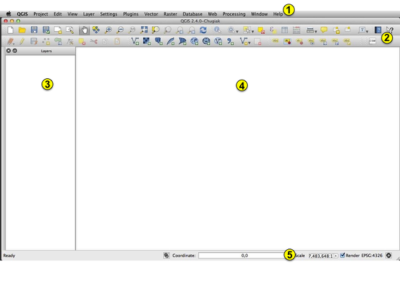
1. Menu bar: provides access to various QGIS features.
2. Toolbar: provides access to most of the same functions as the menus.
3. This area lists all the layers in the project.
4. Map view: maps are displayed in this area.
5. Status Bar: The status bar shows you your current position in map coordinates as the mouse pointer is moved across the map view.

4. Starting a new project

Go to menu Project → Save or Project → Save As (the same options are available in the toolbar). Then, choose the name for your project (e.g., my_project) and the location to save it.

5. Loading raster data

Raster data in GIS are matrices of discrete cells that represent features on, above or below the earth’s surface. Each cell in the raster grid is the same size, and cells are usually rectangular (in QGIS they will always be rectangular). Typical raster datasets include remote sensing data such as aerial photography or satellite imagery and modeled data such as an elevation matrix.

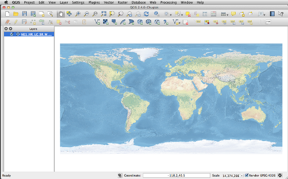
Raster layers are loaded either by clicking on the Add Raster Layer icon on the toolbar or by selecting the Layer → Add Raster Layer menu option. The file that we need now is NE1_LR_LC_SR_W_DR.tif. Browse to the folder where you saved the file, and click the button [Open]. You might be asked to select the correct projection for this layer; in this case, select WGS 84, and click [OK]. Now, on the Map view area, you should see a topographical world map, like this:

On the toolbar, select the function Pan Map; this function is used to move the map around. Also, use or to Zoom In or Zoom Out. On the layers list, uncheck the box and this will make the layer invisible (this is useful when you are working with multiple layers). Now, check the box to make it visible again.

6. Loading shapefiles

Shapefiles describe vector features. Vector data provide a way to represent real world features within the GIS environment. A vector feature has its shape represented using geometry. The geometry is made up of one or more interconnected vertices. A vertex describes a position in space using an X, Y axis.

To load a shapefile, click on the Add Vector Layer toolbar button or, on the menu, select the option Layer → Add Vector Layer. This will bring up a new window. From the available options check File. Click on button [Browse] to navigate the file system and select the shapefile. The file that we need now is world_borders.shp that is inside the folder world_borders. You can also select the Encoding type for the shapefile if desired. For now, choose "System". Then, click the button [Open]. You might be asked to select the correct projection for this layer; in this case, select WGS 84, and click [OK].

A random color is assigned to every layer you add. To change the style of a layer (for instance, to make it more transparent), open the Layer Properties dialog by double clicking on the layer name or by right-clicking on the name in the legend and choosing Properties from the popup menu. Under Style you can change colors and patterns. In the area Symbol layers click on Simple fill; on the right, pick up a new color for Border (choose a color that is easy to distinguish from the raster background, e.g., black) and change the Fill style to No brush. To end editing colors and styles in this layer, click the button [OK]. When you are done, your map should look like this:

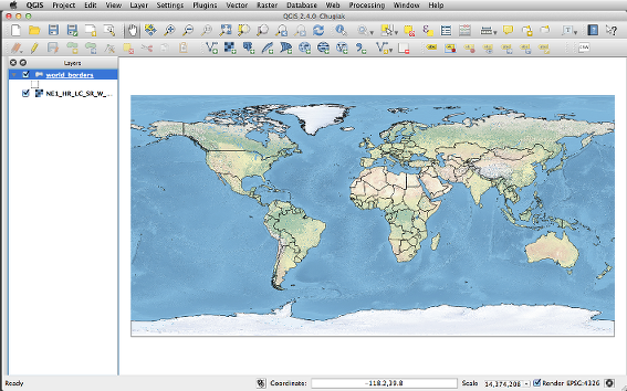
Now that you have two layers, note that a layer can be selected and dragged up or down in the legend to change the z-ordering. Z-ordering means that layers listed nearer the top of the legend are drawn over layers listed lower down in the legend.

It is now time to save your project. Go to menu Project → Save or find the same options on the toolbar. From now on, save your project from time to time.

7. Loading the .csv file containing your species distribution data

We consider that using the species distribution data aids drawing the polygons that represent the user-defined operational areas used for biogeographical analyses; therefore, we will explain how to upload this kind of data below. However, you may prefer to make your polygons without using the species distribution data; if this is the case, go direct to Step 8.

Go to menu Layer → Add Delimited Text Layer or click the toolbar icon Add Delimited Text Layer to open the Create a Layer from a Delimited Text File dialog, and then select the file localities.csv file by clicking on the [Browse] button. Once the file is selected, QGIS attempts to parse the file using the last used delimiter. To properly parse the file, it is important to select the correct delimiter. Under "File format", check "Custom delimiters", and then check the "tab" box. Note that, when using your own data, you may need to select other boxes, depending on the file you have. You may also need to change the Encoding so the program properly reads your file. Make sure that when the program displays the data, the taxon names, the latitude and the longitude data are all in different columns.

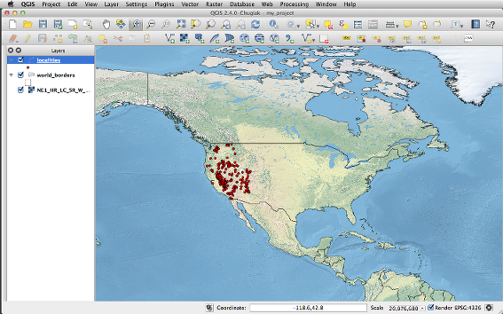
Assign the "X field" (Longitude) and the "Y field" (Latitude), and then click [OK]. The Coordinate Reference System Selector dialog will show up. Leave as it is and click [OK]. You should now see several points on Western USA.

On the Layers list, click on the layer you have just created, and then choose Layer → Save as (or right click on the name of the layer). Click [Browse] to select the place where you want to save the file, then type a name (e.g., "localities"). Then click [OK].

8. Drawing your own polygons

First, zoom in to the area where your points are (or the area of interest, if you are not using your species distribution data). Choose New → New Shapefile Layer from the Layer menu (or the same button on the toolbar). The New Vector Layer dialog will be displayed. Choose the type of layer "polygon". On the Attributes list, select "id", and click the button [Remove attribute]. Under New attribute, type a name (e.g., "my_polygons"), click on [Add to attribute list], and then click [OK]. You will be prompted to the Save as dialog. Type the file name ("my_polygon") and click [Save]. You will be able to see the new layer in the Layers list.

Click on the layer name to select the layer you have just created. All editing sessions start by choosing the Toggle editing option (either on the toolbar or under the Layer menu). Select this option and note that the little pencil symbol will show up beside the name of the layer, indicating that the layer is now editable. Now, click on the Add Feature icon (or select Edit → Add Feature). When you do this, the cursor will look different (not an arrow head). Left-click on the map area to create the first point of your new feature. Keep on left-clicking for each additional point you wish to include in your polygon. When you have finished adding points (i.e., the polygon represents the desired operational area), right-click anywhere on the map area to confirm you have finished entering the geometry of that feature. The attribute window will appear. Input the name you want for your polygon (e.g.,"polygon1"), and click [OK]. Then, click on Save Layer Edits (either on the toolbar or under the Layer menu).

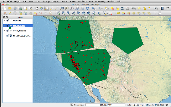
For this example, create three polygons in the same layer: one encompassing the points at the North, another polygon in the Southern area, and one polygon that does not encompass the species points/distribution, like this, for example:

You can edit the shape of a polygon with the Node tool. First, click on the icon on the toolbar, and select "Select Single Feature". Then, click on the polygon you want to reshape; the change of color of the polygon indicates this feature is now selected. Next, on the toolbar, click on the Node tool to make the vertices editable; then click on one of the vertices of your polygon (the vertices will become more evident). Move the vertices (one at a time) until you reach the desired shape. You can also add nodes by double-clicking the outline of the polygon. When you are done editing, unselect the Node Tool, and save your changes. 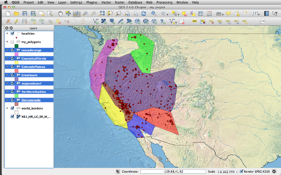Along with all the example files, we are also providing some pre-made polygons (polygons_shapefiles folder) that represent operational areas for our example, so you can see how to draw your polygons when working with your own data set. For uploading these shape files, repeat the instructions described under Step 6.

9. Extract information from your polygons

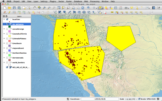
Make the layer with your polygons active by clicking on it in the layers list. Use the tool to select the features on the source layer. For this example, choose Select features by rectangle. Click on the map and draw a rectangle, for selecting all your polygons at once. When the polygons are selected, they will become yellow.

Choose Edit → Copy Features from the Edit menu (also <control + C> in Windows/Linux or <command + C> in Mac computers). Then, paste it on a blank text document. Save the file as "Unix line breaks". The text should look like this:

This file is now ready for use in SpeciesGeoCoder.