Tutorial 04: Double-Mach Reflection

Tutorial Goal

In this tutorial, the setup of an unsteady, inviscid, single-species simulation in a two-dimensional domain is demonstrated. The following capabilities of HAMeRS will be shown:

• Sixth-order shock capturing method WCNS6-LD
• Multiple levels of adaptive mesh refinement using Jameson sensor on density field to identify regions for refinement
• User-defined special boundary conditions

Problem Description

This is a non-dimensional single-species benchmark problem suggested by Woodward and Colella. The initial conditions of the problem is:

Initial Conditions and Special Boundary Conditions

The file containing the initial conditions of this problem (DoubleMachReflection2D.cpp) can be found in problems/Euler/initial_conditions and the initial conditions should be set up by ln -sf <absolute path to DoubleMachReflection2D.cpp> src/apps/Euler/EulerInitialConditions.cpp. The file containing the special boundary conditions of this problem (DoubleMachReflection2D.cpp) can be found in problems/Euler/boundary_conditions and the special boundary conditions should be set up by ln -sf <absolute path to DoubleMachReflection2D.cpp> src/apps/Euler/EulerSpecialBoundaryConditions.cpp. The code has to be re-compiled after the links to the actual initial condition and special boundary condition files are set.

Input File Configurations

The configurations of the input file are discussed in this section. Only settings of several important blocks are discussed. The first thing to choose in the input file is whether it is an Euler (inviscid) or Navier-Stokes (diffusive and viscous) application. Since our problem is inviscid, we first set the application type to be Euler:

Application = "Euler"

The next thing to set is the block Euler:

Euler
{
    // Name of project
    project_name = "2D double-Mach reflection"

    // Number of species
    num_species = 1

    // Flow model to use
    flow_model = "SINGLE_SPECIES"

    Flow_model
    {
        // Equation of state to use
        equation_of_state = "IDEAL_GAS"

        Equation_of_state_mixing_rules
        {
            species_gamma = 1.4
            species_R = 1.0
        }
    }

    // Convective flux reconstructor to use
    convective_flux_reconstructor = "WCNS6_LD_HLLC_HLL"

    Convective_flux_reconstructor{}

    Boundary_data
    {
        // Set the boundary conditions for edges
        boundary_edge_xlo
        {
            boundary_condition = "DIRICHLET"
            density            = 8.0
            velocity           = 7.144709581, -4.125
            pressure           = 116.5
        }

        boundary_edge_xhi
        {
            boundary_condition = "FLOW"
        }

        boundary_edge_ylo
        {
            boundary_condition = "REFLECT"
        }

        boundary_edge_yhi
        {
            boundary_condition = "REFLECT"
        }

        // Set the boundary conditions for nodes
        boundary_node_xlo_ylo
        {
            boundary_condition = "XDIRICHLET"
            density            = 8.0
            velocity           = 7.144709581, -4.125
            pressure           = 116.5
        }

        boundary_node_xhi_ylo
        {
            boundary_condition = "XFLOW"
        }

        boundary_node_xlo_yhi
        {
            boundary_condition = "XDIRICHLET"
            density            = 8.0
            velocity           = 7.144709581, -4.125
            pressure           = 116.5
        }

        boundary_node_xhi_yhi
        {
            boundary_condition = "XFLOW"
        }
    }

    Gradient_tagger
    {
        gradient_sensors = "JAMESON_GRADIENT"

        JAMESON_GRADIENT
        {
            Jameson_gradient_variables = "DENSITY"

            Jameson_gradient_tol = 2.0e-2
        }
    }
}

Dirichlet boundary conditions are specified for the left boundary. The values of the primitive variables at the left boundary are set. Constant extrapolation is used for ghost cells at the right boundary. The boundary conditions of the lower and upper boundaries are set to "REFLECT" arbitrarily since the actual boundary conditions are replaced by the special boundary conditions.

The settings for Main is very similar to those of tutorial 1 and are not discussed.

The following settings are used for CartesianGeometry:

CartesianGeometry
{
    // Lower and upper indices of computational domain
    domain_boxes = [(0, 0), (239, 59)]
    x_lo         = 0.0, 0.0 // Lower end of computational domain
    x_up         = 4.0, 1.0 // Upper end of computational domain

    // Periodic dimension. A non-zero value indicates that the direction is periodic
    periodic_dimension = 0, 0
}

The following settings are used for ExtendedTagAndInitialize:

ExtendedTagAndInitialize
{
    // Tagging method for refinement to use
    tagging_method = "GRADIENT_DETECTOR"
}

The parameters of adaptive mesh refinement are set in PatchHierarchy. In this tutorial, the maximum number of mesh levels is set to 3 and all levels have the same refinement ratio to coarser levels.

PatchHierarchy
{
    // Maximum number of levels in hierarchy
    max_levels = 3

    ratio_to_coarser
    {
        // Vector ratio to next coarser level
        level_1 = 2, 2 // all finer levels will use same values as level_1...
    }

    largest_patch_size
    {
        level_0 = 1000, 1000 // all finer levels will use same values as level_0...
    }

    smallest_patch_size
    {
       level_0 = 4, 4 // all finer levels will use same values as level_0...
    }
}

The following settings are used for RungeKuttaLevelIntegrator and TimeRefinementIntegrator:

RungeKuttaLevelIntegrator
{
    cfl                      = 0.4e0 // Max cfl factor used in problem
    cfl_init                 = 0.4e0 // Initial cfl factor
    lag_dt_computation       = FALSE
    use_ghosts_to_compute_dt = TRUE
}

TimeRefinementIntegrator
{
    start_time           = 0.0e0  // Initial simulation time
    end_time             = 2.0e-1 // Final simulation time
    grow_dt              = 1.0e0  // Growth factor for timesteps
    max_integrator_steps = 10000  // Max number of simulation timesteps
    tag_buffer           = 2, 2   // array of integer values (one for each level that
                                  // may be refined representing the number of cells
                                  // by which tagged cells are buffered)
}

The tag_buffer inside TimeRefinementIntegrator represents the number of cells by which tagged cells are buffered before clustering into boxes.

Running HAMeRS

To run the simulation with one core, first put the input file inside a directory named tutorial_04 under HAMeRS. Then, execute the built main executable inside build/src/exec/main with the input file:

../build/exec/main <input filename>

To run the simulation with multiple cores, you can try mpirun/mpiexec/srun, depending on the MPI library used for the compilation of HAMeRS. For example, if mpirun is used:

mpirun -np <number of processors> ../build/src/exec/main <input filename>

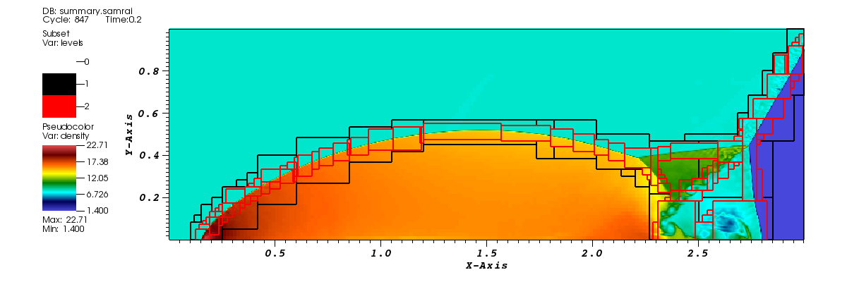
Visualization Using VisIt

The data can be visualized by opening dumps.visit inside the viz folder with VisIt.The figure below shows the density field and refined regions at the end of simulation generated from VisIt. The black and red boxes show the second and third levels of meshes respectively: