How to measure the areas of the grain profiles with ImageJ - marcoalopez/GrainSizeTools GitHub Wiki
[!WARNING] This tutorial assumes that you have installed the ImageJ application. If this is not the case, go here to download and install it. You can also install different flavours of the ImageJ application that will work similarly (see here for a summary).
As a cautionary note, this is not a detailed tutorial on image analysis methods using ImageJ, but a quick systematic tutorial on how to measure the areas of the grain profiles from a thin section to later estimate the grain size and grain size distribution using the GrainSizeTools script. If you are interested in image analysis methods (e.g. grain segmentation techniques, shape characterization, etc.) you should have a look at the list of references at the end of this tutorial.
Previous considerations on Grain Maps
Grain size in rocks is usually measured from sections (2D data, i.e. apparent grain size) using image analysis techniques, resulting in grain boundary maps similar to the one shown below
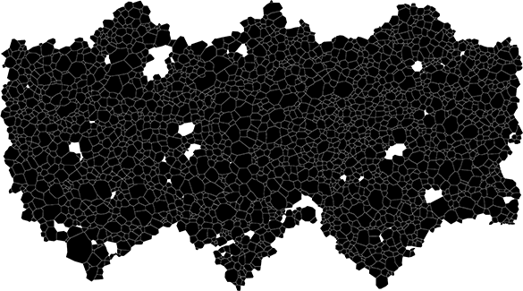
Figure 1. A grain boundary/size map
Briefly, the grain size maps used to calculate the grain size are binary images, where only two possible values exist, 0 for black pixels (the grains) and 1 for white pixels (the grain boundary). The list of techniques that allow the transition from a raw image to a grain boundary/size map, known as grain segmentation and binarization, is extensive and highly dependent on the image source. A discussion of these grain segmentation methods is beyond the scope of this tutorial and the reader is referred to the two references cited at the end of this section. Instead, this tutorial will focus on showing, in a very general way, some things to keep in mind when working with binary grain maps and how to perform basic measurements using the ImageJ software.
Once the grain segmentation is done, it is crucial to ensure that the pixel boundaries of the grains are at least two or three pixels wide (Fig. 2). This will prevent the formation of unwanted artefacts, since if two black pixels belonging to two different grains are placed next to each other, both grains will be considered to be the same grain by the image analysis software.
Figure 2. Detail of grain boundaries in a binary grain map. The figure shows the boundaries (in white) between three grains in a grain boundary map. The squares represent the pixels in the image. The boundaries are two to three pixels wide approximately.
[!CAUTION] Be sure to track the resolution of the image at each step, from the raw image you get from the microscope to the final binary grain map on which you will make the measurements. Knowing the size of the pixels is essential and will allow you to set the scale of the image to correctly measure the areas of the grain sections.
[!TIP] Although the following section only shows how to measure grain size from binary grain maps, if you are working with optical images you can do all the pre-processing, i.e. segmentation and binary image creation, within the ImageJ application.
Measuring the areas of the grain profiles
-
Open the grain boundary map with the ImageJ application
-
To measure the areas of the grain profiles it is first necessary to convert the grain boundary map into a binary image. If this was not done previously, go to
Process>Binaryand click onMake binary. Also, make sure that the areas of grain profiles are in black and the grain boundaries in white and not the other way around. If not, invert the image inEdit>Invert. -
Then, it is necessary to set the scale of the image. Go to
Analize>Set Scale. A new window will appear (Fig. 3). To set the scale, you need to know the size of a feature, such as the width of the image, or the size of an object such as a scale bar. The size of the image in pixels can be check in the upper left corner of the window, within the parentheses, containing the image. To use a particular object of the image as scale the procedure is: i) Use the line selection tool in the toolbar (Fig. 3) and draw a line along the length of the feature or scale bar; ii) go toAnalize>Set Scale; iii) the distance of the drawn line in pixels will appear in the upper box, so enter the dimension of the object/scale bar in the 'known distance' box and set the units in the 'Unit length' box; iv) do not check 'Global' unless you want that all your images have the same calibration and click ok. Now, you can check in the upper left corner of the window the size of the image in microns (millimetres or whatever) and pixels.
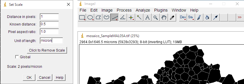
Figure 3. At left, the Set Scale window. In the upper right, the ImageJ menu and tool bars. The line selection tool is the fifth element from the left (which is actually selected). In the bottom right, the upper left corner of the window that contains the grain boundary map. The numbers are the size in microns and the size in pixels (in brackets).
-
The next step requires to set the measurements to be done. For this, go to
Analize>Set Measurementsand a new window will appear. Make sure that 'Area' is selected. You can also set at the bottom of the window the desired number of decimal places. Hit ok. -
To measure the areas of our grain profiles we need to go to
Analize>Analize Particles. A new window will appear with different options (Fig. 4). The first two are for establishing certain conditions to exclude anything that is not an object of interest in the image. The first one is based on the size of the objects in pixels by establishing a range of size. We usually set a minimum of four pixels and the maximum set to infinity to rule out possible artefacts hard to detect by the eye. This ultimately depends on the quality and the nature of your grain boundary map. For example, people working with high-resolution EBSD maps usually discard any grain with less than ten pixels. The second option is based on the roundness of the grains. We usually leave the default range values 0.00-1.00, but again this depends on your data and purpose. For example, the roundness parameter could be useful to differentiate between non-recrystallized and recrystallized grains in some cases. Just below, the 'show' drop-down menu allows the user to obtain different types of images when the particle analysis is done. We usually set this to 'Outlines' to obtain an image with all the grains measured outlined and numbered, which can be useful later to check the data set. Finally, the user can choose between different options. In our case, it is just necessary to select 'Display results'. Hit ok.
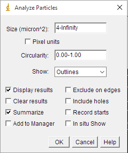
Figure 4. Analyze particles window showing the different options
- After a while, several windows will appear. At least, one containing the results of the measures (Fig. 5), and others containing the image with the grains outlined and numbered. Note that the numbers displayed within the grains in the image correspond to the values showed in the first column of the results. To save the image go to the ImageJ menu bar, click on
File>Save As, and choose the file type you prefer (we encourage you to use PNG or TIFF for such type of image). To save the results we have different options. In the menu bar of the window containing the results, go toResults>Optionsand a new window will appear (Fig. 6). In the third line, you can choose to save the results as a text (.txt), CSV comma-separated (.csv) or Excel (.xls) file types. We encourage you to choose either txt or CSV since both are widely supported formats to exchange tabular data. Regarding the 'Results Table Options' at the bottom, make sure that 'Save column headers' are selected since this headers will be used by the GrainSizeTools script to automatically extract the data from the column 'Area'. Finally, in the same window go toFile>Save Asand choose a name for the file. You are done.
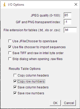
Figure 6. ImageJ I/O options window.
List of useful references
Note: This list of references is by no means exhaustive. It simply reflects some books, articles or websites that I find interesting on the subject. I intend to extend this list over time. Regarding the ImageJ/Fiji application, there are many books and tutorials available on the web.
Russ, J.C., 2011. The image processing handbook. CRC Press. Taylor & Francis Group
This is a general-purpose book on image analysis written by professor John C. Russ from the Material Sciences and Engineering at North Carolina State University. Although the book is not specifically focused on structural geology, thin sections, or even rocks, it covers a wide variety of procedures in image analysis and contains very nice examples of image enhancement, segmentation techniques or shape characterization. I find the text very clear and well-written, so if you are looking for a general-purpose image analysis book, this is the best one I know.
Heilbronner, R., Barret, S., 2014. Image Analysis in Earth Sciences. Springer-Verlag Berlin Heidelberg. https://doi.org/10.1007/978-3-642-10343-8
This book focuses on image analysis related to Earth Sciences putting much emphasis on methods used in structural geology. The first two chapters deal with image processing and grain segmentation techniques using the software Image SXM, which is a different flavour of the ImageJ family applications (see here).