Topographic Mapping - ucdavis/erplab GitHub Wiki

Topographic Mapping

ERPLAB provides a simple interface into EEGLAB's topographic mapping functions, which you will access by selecting ERPLAB > Plot ERP > Plot ERP Scalp Maps. This routine allows you to plot the data from one or more time period for a selected set of bins from the currently selected ERPset. The GUI is shown below, along with an example of the output.

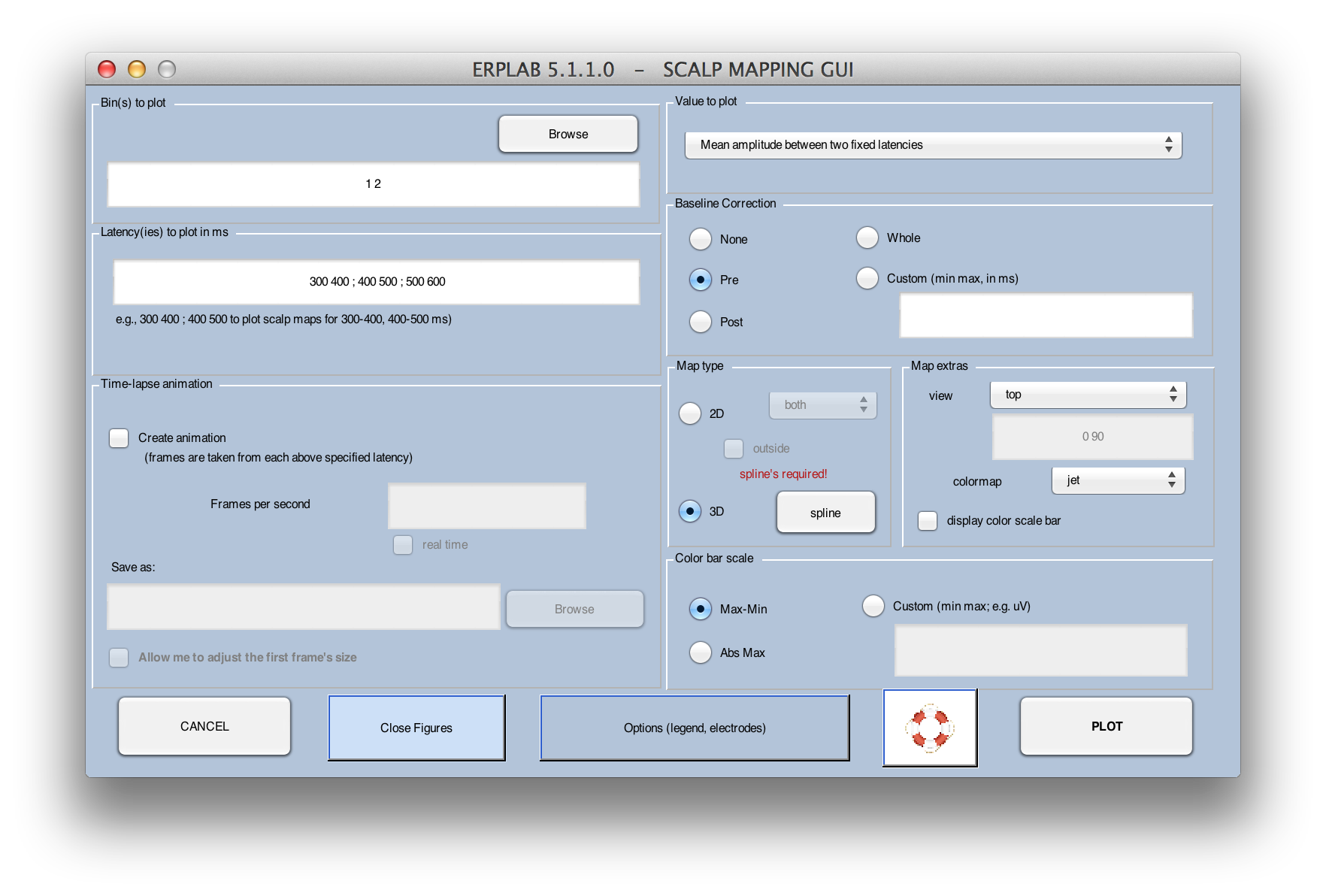
To plot a set of topographic maps, you start by selecting what kinds of values to plot. The options are:

Instantaneous amplitude- The amplitude at a single time point (e.g., 300 ms)

Mean amplitude between two fixed latencies- The mean voltage in a time period (e.g., 300-400 ms)

Instantaneous amplitude Laplacian- Surface Laplacian plot of instantaneous amplitude

Mean amplitude between two fixed latencies- Surface Laplacian plot of mean amplitude

Root mean square value- This is the RMS voltage over a specified time range

For instantaneous amplitude, you provide a set of one or more latencies in the Latencies to plot text box (e.g., "100 150 200 250 300" or equivalently "100:50:300"). For mean or RMS amplitude, you provide one or more sets of time periods. For example, you would specify 300 450 to plot the scalp distribution of the mean voltage between 300 and 450 ms. You can also specify multiple time periods, separated by semicolons (e.g., "200 300 ; 300 400; 400 500" to plot maps of mean amplitude from 200-300, 300-400, and 400-500).

There are several options for determining the scale of the maps. If you select Max-Min, the routine automatically chooses a scale for each bin on the basis of the minimum and maximum voltages found in that bin (e.g., the chosen scale might go from -4 µV to +9 µV). If you select Abs Max, the routine finds the minimum and maximum values, and creates a symmetrical scale depending on which has a greater absolute value (e.g., the chosen scale might go from -9 µV to +9 µV). For these two options, each bin is scaled separately. A third option is Custom, which allows you to specify the minimum and maximum values (e.g., you might put -5 +5 in the text box). In this case, the scale is the same for each bin. There are a variety of additional plotting options (e.g., turning on or off electrode markers) that are accessed with the Options button.

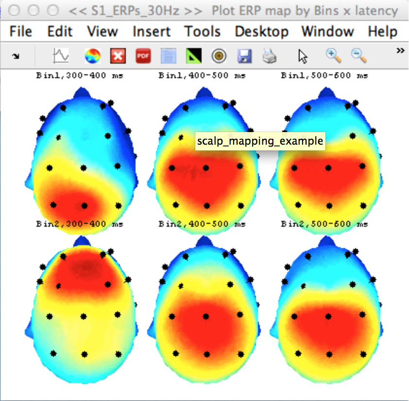
You can also choose between 2D maps (which always use a top viewpoint) and 3D maps (which allow you to specify the viewpoint). The following is an example of the 3D maps, using a top viewpoint.

The topographic plotting routine requires that the location of each electrode is specified (not just the name, but the 3-D coordinates). EEGLAB provides a set of tools for setting the electrode locations in the current EEG structure, accessed via Edit > Channel Locations, and this can be done very easily by using a set of standard coordinates based on the electrode names. Ordinarily, you will do this prior to averaging. If, however, you select ERPLAB > Plot ERP > Plot ERP Scalp Maps without first setting the channel locations, ERPLAB will allow you to use EEGLAB's channel location GUI to set the channel locations within the current ERP structure (see the screenshots below). We typically find that we can simply accept the default settings.

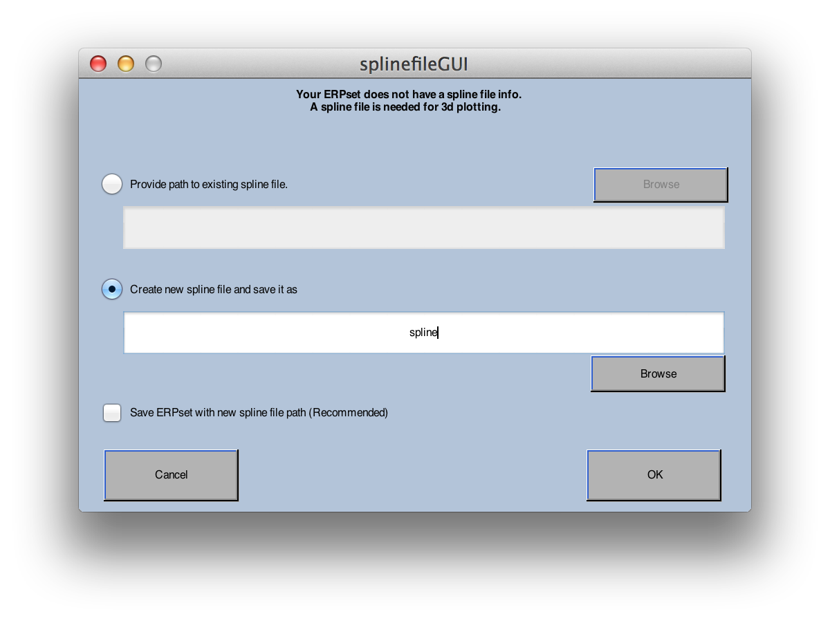
Plotting a 3D topo maps requires creating a spline file (which is used in the interpolation of values across the model head). If you haven't yet plotted the data from a given ERPset, you probably won't have a spline file associated with it. If this happens, you will get the window shown in the screenshot below. If you've already created a spline file for this set of electrodes, you can specify its location. If you haven't already created the spline file, you will tell it to create a new one and give a name for the file. If you check Save ERPset with new spline file path to disk, it will save a new version of your ERPset with information about how to find the spline file in the future.