This phase analysis variables' liveness which information will be used in Register Allocation phase(because we assume there as many as possible registers in the former phase, and actually we have to make these ideal registers fit in a limited number of registers).

We say a variable is live if it holds a value that may be needed in the future, so this analysis is called liveness analysis.

Let's take some arithmetic operations for example(thought non-formal):

1. a = a + b
2. b = b * b
3. c = c + b

In the code above, variable a is only used in statement 1, variable c is only used in statement 3 and variable b is used both in statement 2 and 3. So, the entire liveness is:

a  ->  1
b  ->  1, 2, 3
c  ->  3

We can obviously see find that the liveness of variable a and c is not interfered, thus, when using registers to store variables we can use the same register to hold a and c which makes used register numbers decreased by one.

To perform analyses on a program, we need to make a control flow graph for it.

Because assembly language code is generally written in sequence and run in sequence, so each statement is represented by one node in the graph and the control flow is expressed by edges between nodes.

Liveness of variables "flows" around the edges of the control-flow graph; determining the live range of each variable is an example of a dataflow problem.

A flow-graph node has out-edges that lead to successor nodes, and in-edges that come from predecessor nodes. The set pred[n] is all the predecessors of node n, and succ[n] is the set of successors.

An assignment to a variable or temporary defines that variable. An occurrence of a variable on the right-hand side of an assignment (or in other expressions) uses the variable. We can speak of the def of a variable as the set of graph nodes that define it; or the def of a graph node as the set of variables that it defines; and similarly for the use of a variable or graph node.

A variable is live on an edge if there is a directed path from that edge to a use of the variable that does not go through any def. A variable is live-in at a node if it is live on any of the in-edges of that node; it is live-out at a node if it is live o any of the out-edges of the node.

However, if found it a little difficult to figure out what it means, but it doesn't matter (-_-).

Terminologies listed above is under arithmetic context. However, assembly instructions have different syntax:

Arithmetics				Machime Instructions
	a = a + b				add 	a, b
	a = a / b				idiv	b

While generating liveness informations (defs and uses), you have to translate instruction meanings into arithmetic meanings. Be careful!

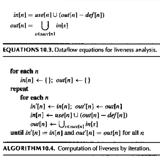
Liveness information (live-in and live-out) can be calculated from use and def as follows:

• If a variable is in use[n], then it is live-in at node n. That is, if a statement uses a variable, the variable is live on entry to that statement.
• If a variable is live-in at node, then it is live-out at all nodes m in pred[n].
• If a variable is live-out at node n, and not in def[n], then the variable is also live-in at n. That is, if someone needs the value of a at the end of statement n, and n does not provide that value, then a's value is needed even on entry to n.

From the figure above we can find that liveness information of one node is dependent of successor nodes. Generally speaking, if statements are executed in sequence, then out[n] is calculated from in[n + 1], and in[n+ 1] is calculated from out[n + 1]. That means if we calculate liveness information from bottom to top, we can make the loop times as few as possible.

However, there are still many control flows in assembly language. So, one node may contains plenty of successors which makes this calculate order difficult to carry out. To make things simple, we just calculate liveness information from the last statement to the first.

When all liveness information (outs and ins) not changed, the calculation is ended.

This algorithm is a conservative approximation and any solution to the dataflow equations is a conservative approximation.

If the value of variable a will truly be needed in some execution of the program when execution reaches node n of the flow graph, then we can be assured that a is live-out at node n in any solution of the equations. But the converse is not true; we might calculate that d is live-out, but that doesn't mean that its value will really be needed.

Although not ideal, this is enough in practice.

To make jobs in Register Allocation simple, we generate an interference graph and a set of MOVE nodes in this phase.

An interference graph is made up of a undirected graph. For register allocations, every register stands for a node, and an interference is represented by an edge between nodes. Under this condition, interference is caused by overlapping live ranges. If a condition that prevents two variables being allocated to the same register, then it causes an interference.

And we have to treat MOVE instructions specially, because MOVEs may or may not stand for interference (two operand registers may be allocated the same register).

Therefore, the way to add interference edges for each new definition is:

• At any nonmove instruction that defines a variable a, where the live-out variables are b1,...,bj, add interference edges (a, b1),...,(a, bj).
• At a move instruction a <- c, where variables b1,...,bj are live-out, add interference edges (a, bj),...,(a, bj) for any bi that is not the same as c.

Support for directed graph:

• myDirectedGraph.h
• myDirectedGraph.cpp

Support for control flow graph:

• myCFGraph.h
• myCFGraph.h

Support for liveness(include interference graph):

• myLiveness.h
• myLiveness.cpp