The Illustrated BERT, ELMo, and co. (How NLP Cracked Transfer Learning)

BERT is a model that broke several records for how well models can handle language-based tasks. Soon after the release of the paper describing the model, the team also open-sourced the code of the model, and made available for download versions of the model that were already pre-trained on massive datasets. This is a momentous development since it enables anyone building a machine learning model involving language processing to use this powerhouse as a readily-available component – saving the time, energy, knowledge, and resources that would have gone to training a language-processing model from scratch.

The two steps of how BERT is developed. You can download the model pre-trained in step 1 (trained on un-annotated data), and only worry about fine-tuning it for step 2.

Example: Sentence Classification

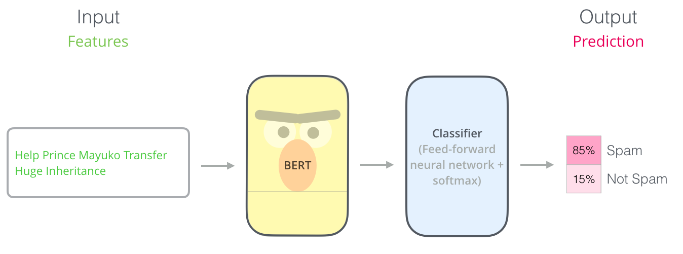
The most straight-forward way to use BERT is to use it to classify a single piece of text. This model would look like this:

To train such a model, you mainly have to train the classifier, with minimal changes happening to the BERT model during the training phase. This training process is called Fine-Tuning, and has roots in Semi-supervised Sequence Learning and ULMFiT.

For people not versed in the topic, since we’re talking about classifiers, then we are in the supervised-learning domain of machine learning. Which would mean we need a labeled dataset to train such a model. For this spam classifier example, the labeled dataset would be a list of email messages and a label (“spam” or “not spam” for each message).

Model Architecture

Now that you have an example use-case in your head for how BERT can be used, let’s take a closer look at how it works.

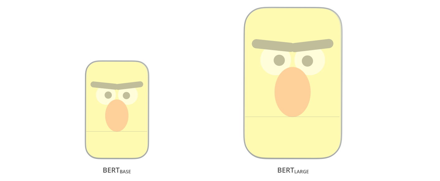
The paper presents two model sizes for BERT:

• BERT BASE – Comparable in size to the OpenAI Transformer in order to compare performance
• BERT LARGE – A ridiculously huge model which achieved the state of the art results reported in the paper

BERT is basically a trained Transformer Encoder stack. The Illustrated Transformer which explains the Transformer model – a foundational concept for BERT and the concepts we’ll discuss next.

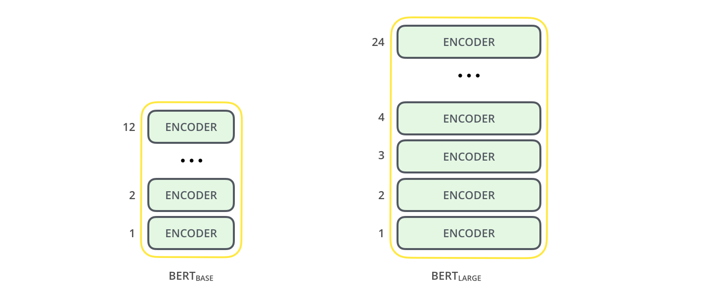
Both BERT model sizes have a large number of encoder layers (which the paper calls Transformer Blocks) – twelve for the Base version, and twenty four for the Large version. These also have larger feedforward-networks (768 and 1024 hidden units respectively), and more attention heads (12 and 16 respectively) than the default configuration in the reference implementation of the Transformer in the initial paper (6 encoder layers, 512 hidden units, and 8 attention heads).

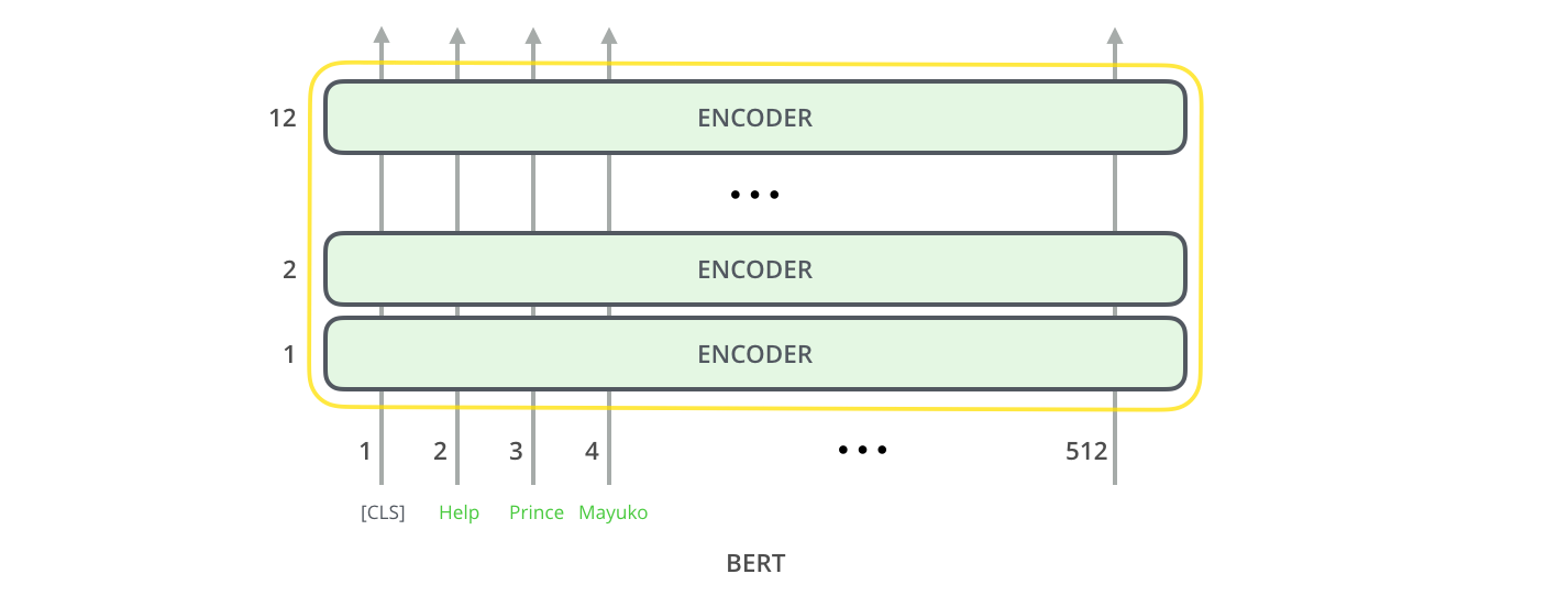
Model Inputs

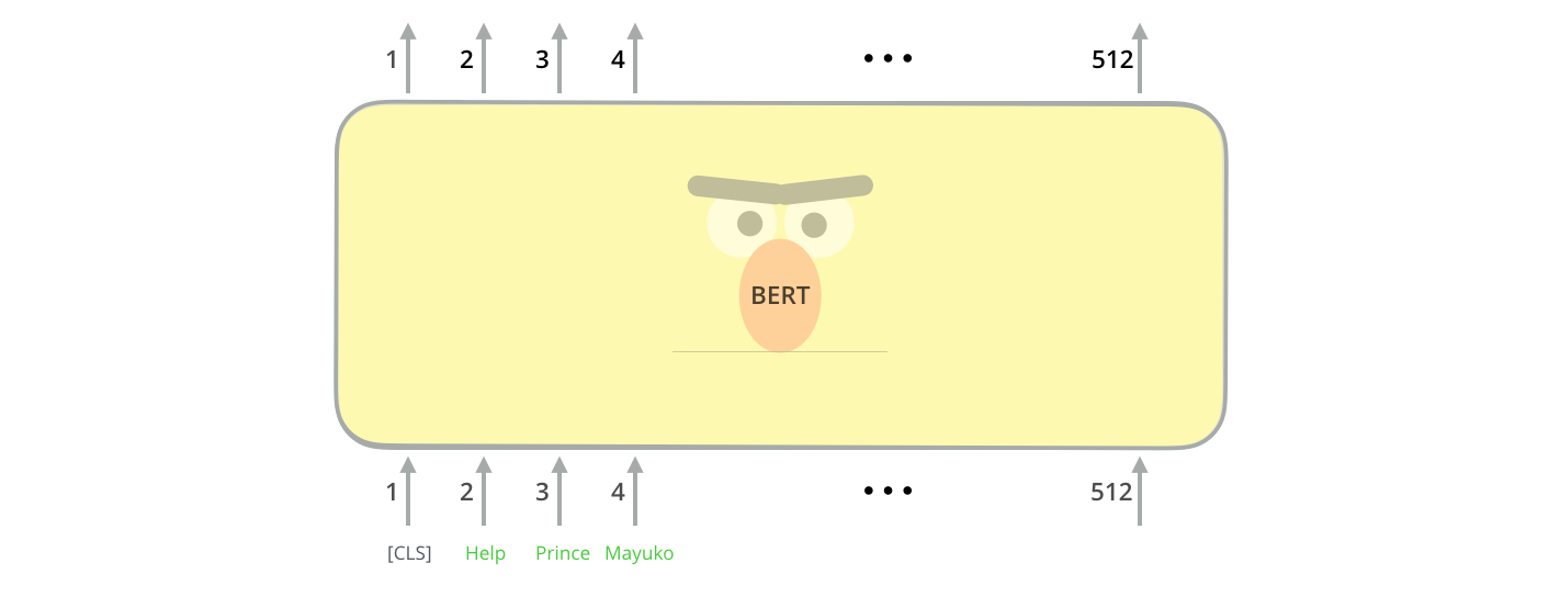
The first input token is supplied with a special [CLS] token for reasons that will become apparent later on. CLS here stands for Classification.

Just like the vanilla encoder of the transformer, BERT takes a sequence of words as input which keep flowing up the stack. Each layer applies self-attention, and passes its results through a feed-forward network, and then hands it off to the next encoder.

In terms of architecture, this has been identical to the Transformer up until this point (aside from size, which are just configurations we can set). It is at the output that we first start seeing how things diverge.

Model Outputs

Each position outputs a vector of size hidden_size (768 in BERT Base). For the sentence classification example we’ve looked at above, we focus on the output of only the first position (that we passed the special [CLS] token to).

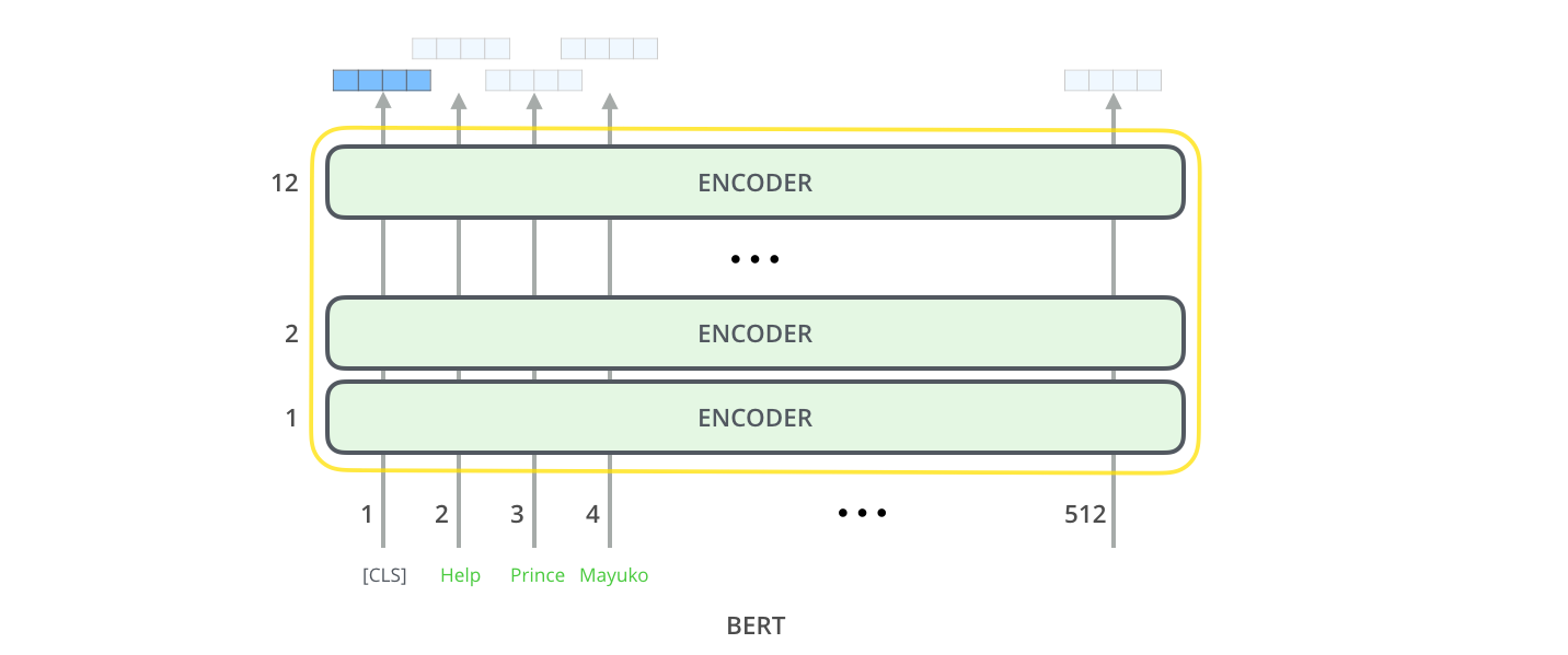
That vector can now be used as the input for a classifier of our choosing. The paper achieves great results by just using a single-layer neural network as the classifier.

If you have more labels (for example if you’re an email service that tags emails with “spam”, “not spam”, “social”, and “promotion”), you just tweak the classifier network to have more output neurons that then pass through softmax.

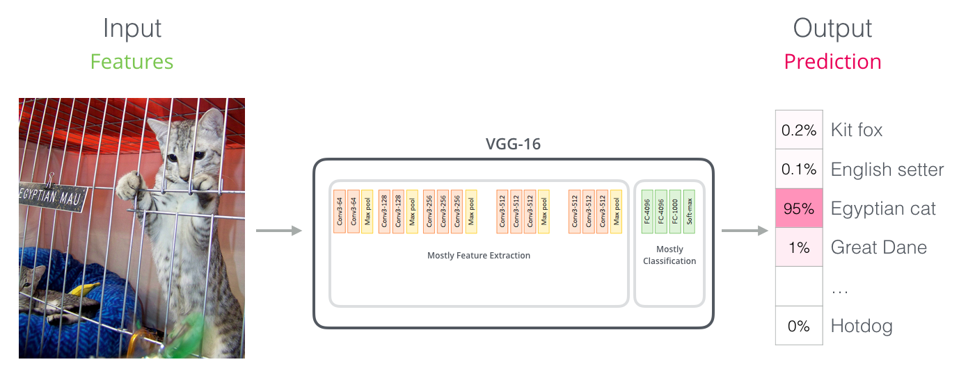
Parallels with Convolutional Nets

For those with a background in computer vision, this vector hand-off should be reminiscent of what happens between the convolution part of a network like VGGNet and the fully-connected classification portion at the end of the network.

A New Age of Embedding

These new developments carry with them a new shift in how words are encoded. Up until now, word-embeddings have been a major force in how leading NLP models deal with language. Methods like Word2Vec and Glove have been widely used for such tasks. Let’s recap how those are used before pointing to what has now changed. This is an example of the GloVe embedding of the word “stick” (with an embedding vector size of 200)

The GloVe word embedding of the word "stick" - a vector of 200 floats (rounded to two decimals). It goes on for two hundred values.

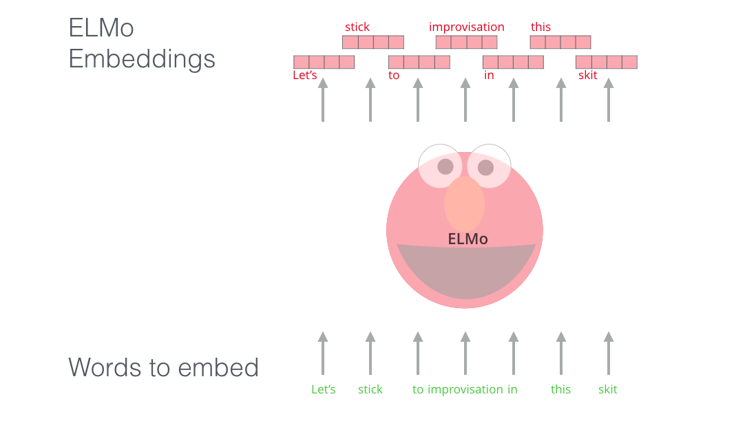
ELMo: Context Matters

If we’re using this GloVe representation, then the word “stick” would be represented by this vector no-matter what the context was. “stick”” has multiple meanings depending on where it’s used. Why not give it an embedding based on the context it’s used in – to both capture the word meaning in that context as well as other contextual information?”. And so, contextualized word-embeddings were born.

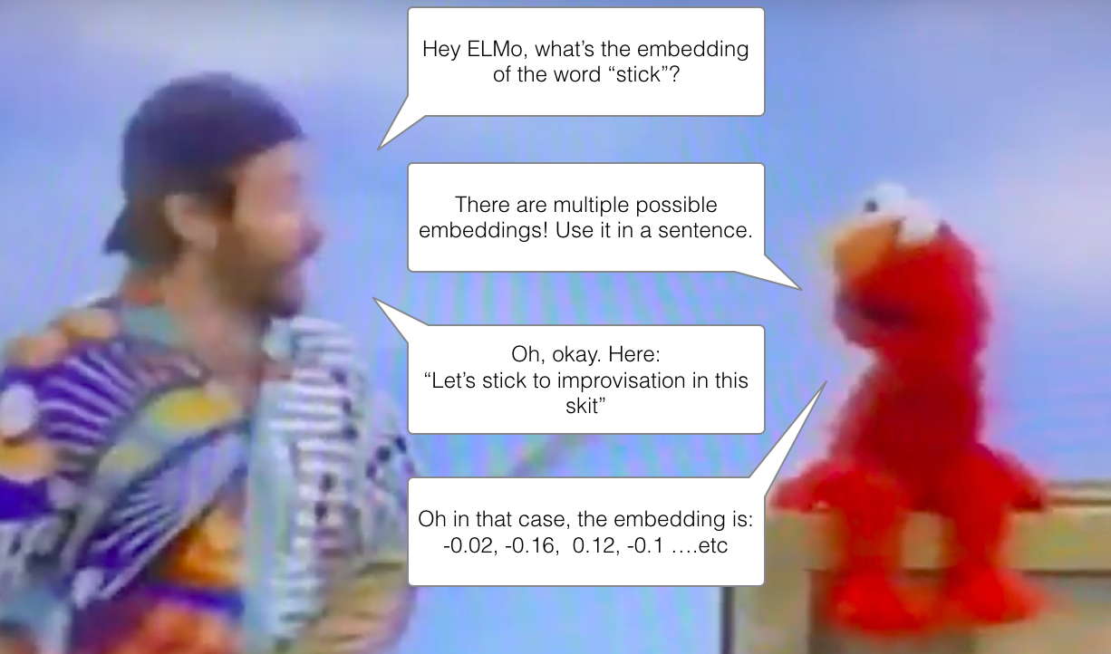
Contextualized word-embeddings can give words different embeddings based on the meaning they carry in the context of the sentence.

Instead of using a fixed embedding for each word, ELMo looks at the entire sentence before assigning each word in it an embedding. It uses a bi-directional LSTM trained on a specific task to be able to create those embeddings.

ELMo provided a significant step towards pre-training in the context of NLP. The ELMo LSTM would be trained on a massive dataset in the language of our dataset, and then we can use it as a component in other models that need to handle language.

What’s ELMo’s secret?

ELMo gained its language understanding from being trained to predict the next word in a sequence of words - a task called Language Modeling. This is convenient because we have vast amounts of text data that such a model can learn from without needing labels.

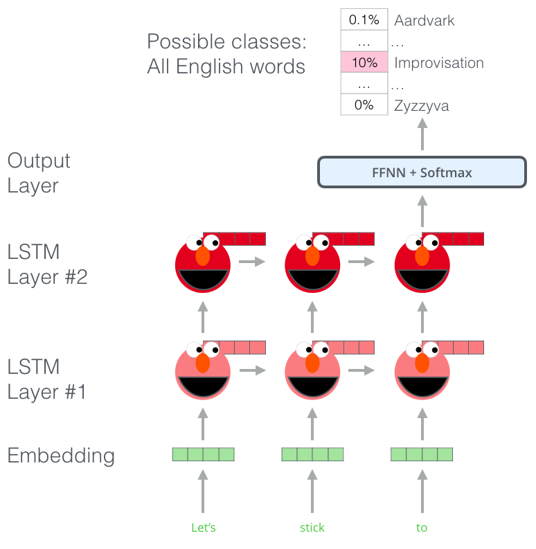
A step in the pre-training process of ELMo: Given “Let’s stick to” as input, predict the next most likely word – a language modeling task. When trained on a large dataset, the model starts to pick up on language patterns. It’s unlikely it’ll accurately guess the next word in this example. More realistically, after a word such as “hang”, it will assign a higher probability to a word like “out” (to spell “hang out”) than to “camera”.

We can see the hidden state of each unrolled-LSTM step peaking out from behind ELMo’s head. Those come in handy in the embedding process after this pre-training is done.

ELMo actually goes a step further and trains a bi-directional LSTM – so that its language model doesn’t only have a sense of the next word, but also the previous word.

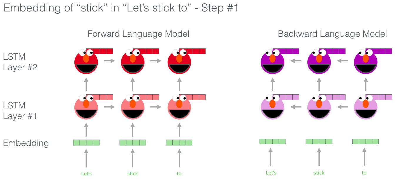
Great slides on ELMo

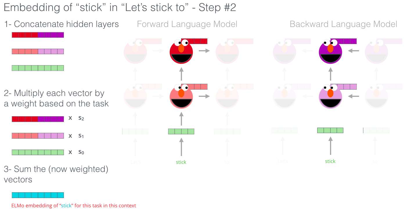
ELMo comes up with the contextualized embedding through grouping together the hidden states (and initial embedding) in a certain way (concatenation followed by weighted summation).

ULM-FiT: Nailing down Transfer Learning in NLP

ULM-FiT introduced methods to effectively utilize a lot of what the model learns during pre-training – more than just embeddings, and more than contextualized embeddings. ULM-FiT introduced a language model and a process to effectively fine-tune that language model for various tasks.

NLP finally had a way to do transfer learning probably as well as Computer Vision could.

The Transformer: Going beyond LSTMs

The Encoder-Decoder structure of the transformer made it perfect for machine translation. But how would you use it for sentence classification? How would you use it to pre-train a language model that can be fine-tuned for other tasks (downstream tasks is what the field calls those supervised-learning tasks that utilize a pre-trained model or component).

OpenAI Transformer: Pre-training a Transformer Decoder for Language Modeling

It turns out we don’t need an entire Transformer to adopt transfer learning and a fine-tunable language model for NLP tasks. We can do with just the decoder of the transformer. The decoder is a good choice because it’s a natural choice for language modeling (predicting the next word) since it’s built to mask future tokens – a valuable feature when it’s generating a translation word by word.

The OpenAI Transformer is made up of the decoder stack from the Transformer

The model stacked twelve decoder layers. Since there is no encoder in this set up, these decoder layers would not have the encoder-decoder attention sublayer that vanilla transformer decoder layers have. It would still have the self-attention layer, however (masked so it doesn’t peak at future tokens).

With this structure, we can proceed to train the model on the same language modeling task: predict the next word using massive (unlabeled) datasets. Just, throw the text of 7,000 books at it and have it learn! Books are great for this sort of task since it allows the model to learn to associate related information even if they’re separated by a lot of text – something you don’t get for example, when you’re training with tweets, or articles.

The OpenAI Transformer is now ready to be trained to predict the next word on a dataset made up of 7,000 books.

Transfer Learning to Downstream Tasks

Now that the OpenAI transformer is pre-trained and its layers have been tuned to reasonably handle language, we can start using it for downstream tasks. Let’s first look at sentence classification (classify an email message as “spam” or “not spam”):

How to use a pre-trained OpenAI transformer to do sentence clasification

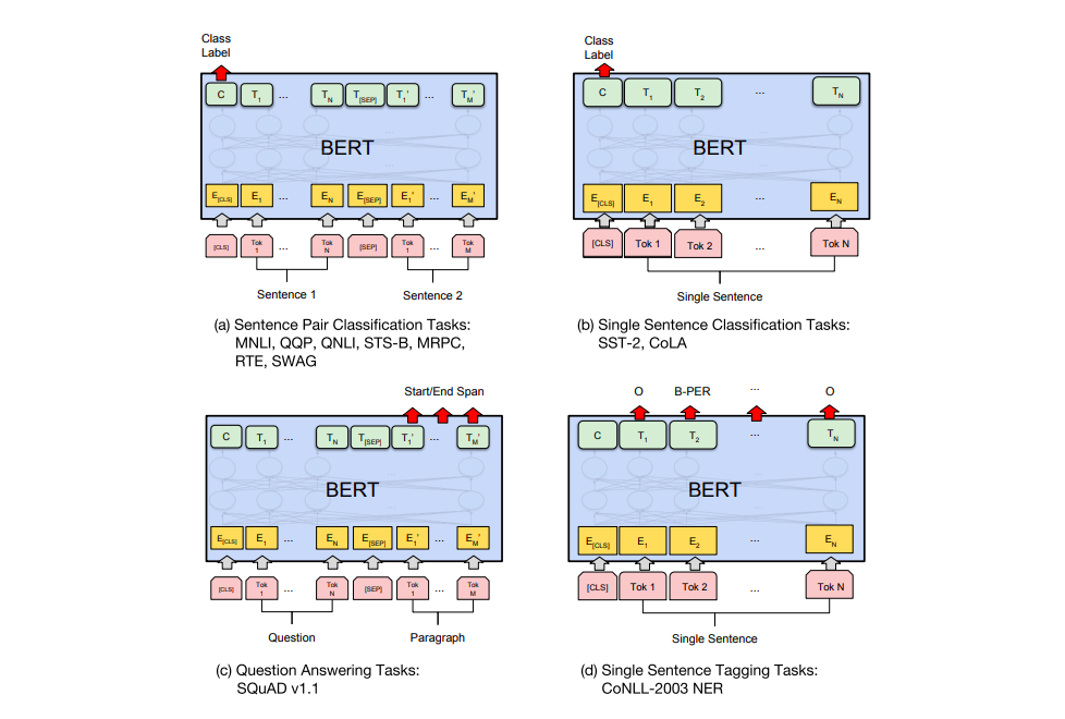
The OpenAI paper outlines a number of input transformations to handle the inputs for different types of tasks. The following image from the paper shows the structures of the models and input transformations to carry out different tasks.

BERT: From Decoders to Encoders

The openAI transformer gave us a fine-tunable pre-trained model based on the Transformer. But something went missing in this transition from LSTMs to Transformers. ELMo’s language model was bi-directional, but the openAI transformer only trains a forward language model. Could we build a transformer-based model whose language model looks both forward and backwards (in the technical jargon – “is conditioned on both left and right context”)?

Masked Language Model

“We’ll use transformer encoders”, said BERT. “We’ll use masks”, said BERT confidently.
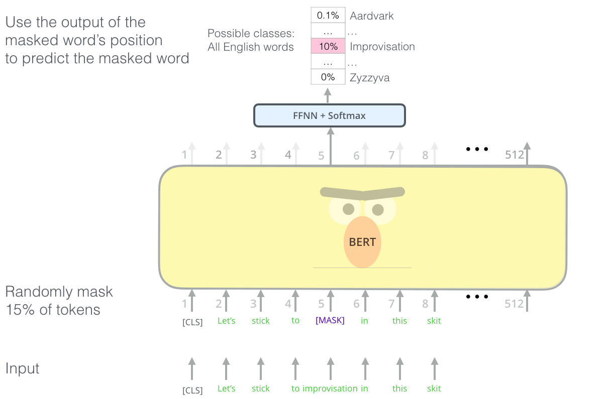
BERT's clever language modeling task masks 15% of words in the input and asks the model to predict the missing word. Finding the right task to train a Transformer stack of encoders is a complex hurdle that BERT resolves by adopting a “masked language model” concept from earlier literature (where it’s called a Cloze task).

Beyond masking 15% of the input, BERT also mixes things a bit in order to improve how the model later fine-tunes. Sometimes it randomly replaces a word with another word and asks the model to predict the correct word in that position.

Two-sentence Tasks

If you look back up at the input transformations the OpenAI transformer does to handle different tasks, you’ll notice that some tasks require the model to say something intelligent about two sentences (e.g. are they simply paraphrased versions of each other? Given a wikipedia entry as input, and a question regarding that entry as another input, can we answer that question?).

To make BERT better at handling relationships between multiple sentences, the pre-training process includes an additional task: Given two sentences (A and B), is B likely to be the sentence that follows A, or not?

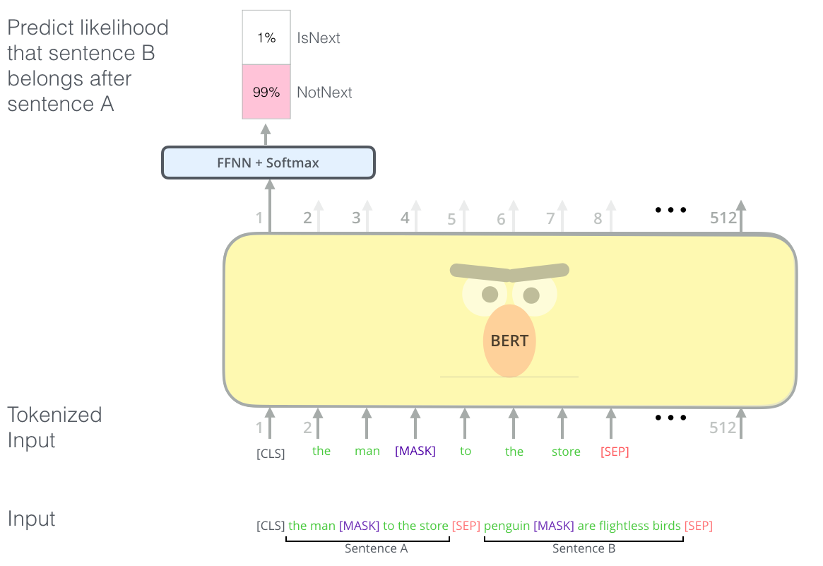
The second task BERT is pre-trained on is a two-sentence classification task. The tokenization is oversimplified in this graphic as BERT actually uses WordPieces as tokens rather than words --- so some words are broken down into smaller chunks.

Task specific-Models

The BERT paper shows a number of ways to use BERT for different tasks.

BERT for feature extraction

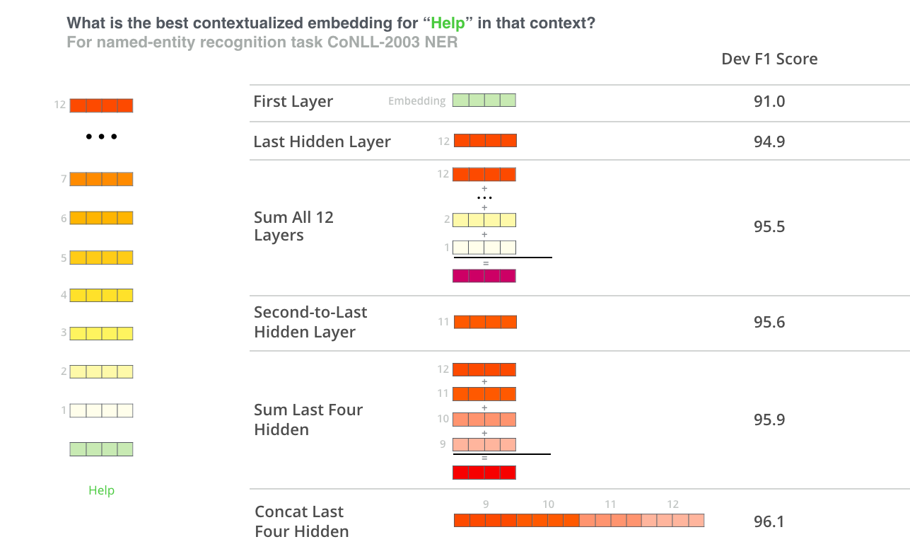
The fine-tuning approach isn’t the only way to use BERT. Just like ELMo, you can use the pre-trained BERT to create contextualized word embeddings. Then you can feed these embeddings to your existing model – a process the paper shows yield results not far behind fine-tuning BERT on a task such as named-entity recognition.

Which vector works best as a contextualized embedding? I would think it depends on the task. The paper examines six choices (Compared to the fine-tuned model which achieved a score of 96.4):

Take BERT out for a spin

The best way to try out BERT is through the BERT FineTuning with Cloud TPUs The next step would be to look at the code in the BERT repo:

• The model is constructed in modeling.py (class BertModel) and is pretty much identical to a vanilla Transformer encoder.

• run_classifier.py is an example of the fine-tuning process. It also constructs the classification layer for the supervised model. If you want to construct your own classifier, check out the create_model() method in that file.

• Several pre-trained models are available for download. These span BERT Base and BERT Large, as well as languages such as English, Chinese, and a multi-lingual model covering 102 languages trained on wikipedia.

• BERT doesn’t look at words as tokens. Rather, it looks at WordPieces. tokenization.py is the tokenizer that would turns your words into wordPieces appropriate for BERT.

You can also check out the PyTorch implementation of BERT. The AllenNLP library uses this implementation to allow using BERT embeddings with any model.

A Visual Guide to Using BERT

Progress has been rapidly accelerating in machine learning models that process language over the last couple of years. This progress has left the research lab and started powering some of the leading digital products. A great example of this is the recent announcement of how the BERT model is now a major force behind Google Search. Google believes this step (or progress in natural language understanding as applied in search) represents “the biggest leap forward in the past five years, and one of the biggest leaps forward in the history of Search”.

This post is a simple tutorial for how to use a variant of BERT to classify sentences. This is an example that is basic enough as a first intro, yet advanced enough to showcase some of the key concepts involved.

Alongside this post, You can the notebook.

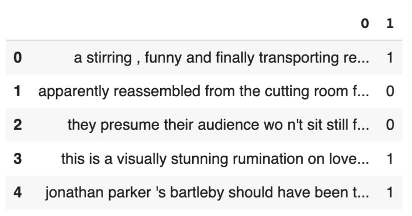
Dataset: SST2

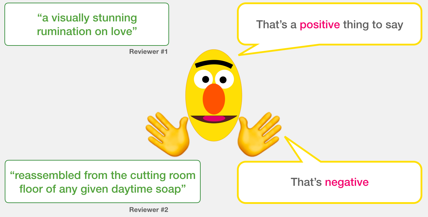
The dataset we will use in this example is SST2, which contains sentences from movie reviews, each labeled as either positive (has the value 1) or negative (has the value 0):

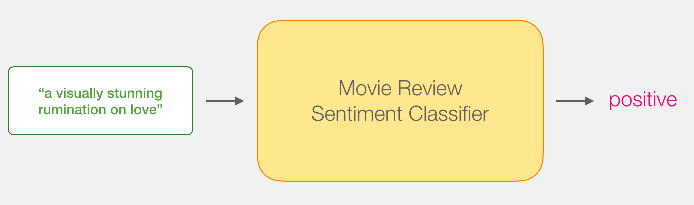
Models: Sentence Sentiment Classification

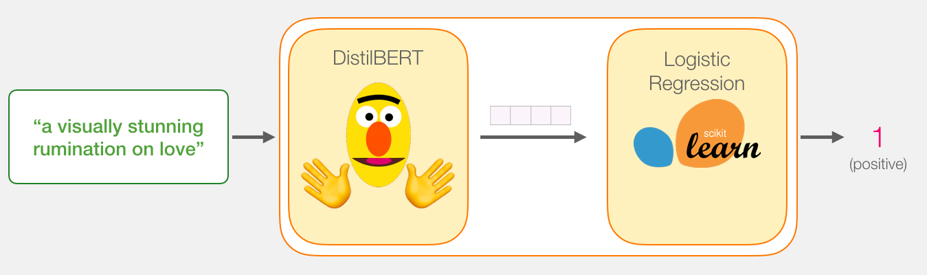
Our goal is to create a model that takes a sentence (just like the ones in our dataset) and produces either 1 (indicating the sentence carries a positive sentiment) or a 0 (indicating the sentence carries a negative sentiment). We can think of it as looking like this:

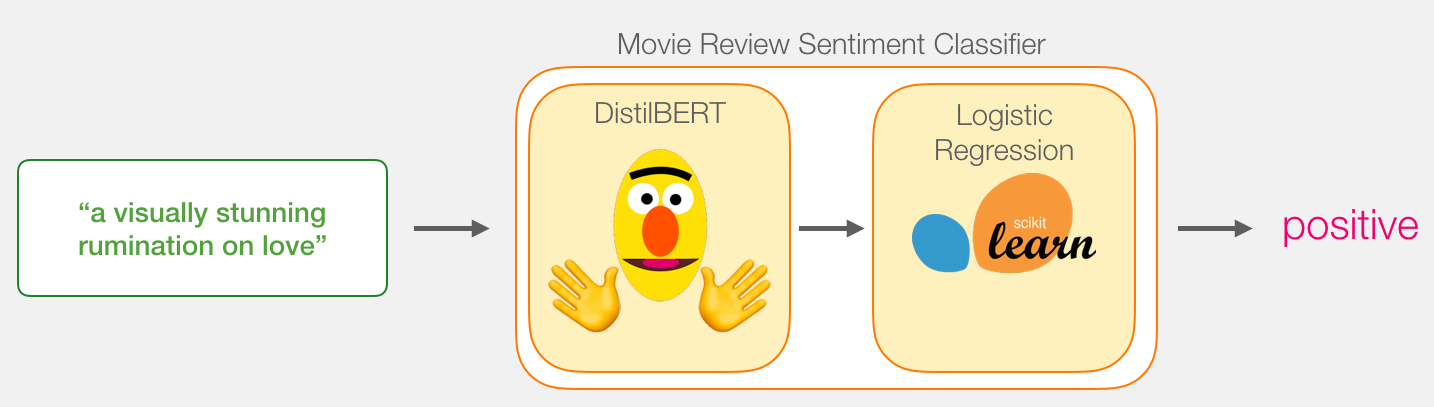
Under the hood, the model is actually made up of two model.

• DistilBERT processes the sentence and passes along some information it extracted from it on to the next model. DistilBERT is a smaller version of BERT developed and open sourced by the team at HuggingFace. It’s a lighter and faster version of BERT that roughly matches its performance.
• The next model, a basic Logistic Regression model from scikit learn will take in the result of DistilBERT’s processing, and classify the sentence as either positive or negative (1 or 0, respectively).

The data we pass between the two models is a vector of size 768. We can think of this of vector as an embedding for the sentence that we can use for classification.

If you’ve read my previous post, Illustrated BERT, this vector is the result of the first position (which receives the [CLS] token as input).

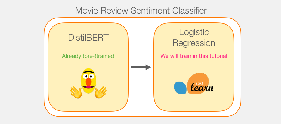
Model Training

While we’ll be using two models, we will only train the logistic regression model. For DistillBERT, we’ll use a model that’s already pre-trained and has a grasp on the English language. This model, however is neither trained not fine-tuned to do sentence classification. We get some sentence classification capability, however, from the general objectives BERT is trained on. This is especially the case with BERT’s output for the first position (associated with the [CLS] token). I believe that’s due to BERT’s second training object – Next sentence classification. That objective seemingly trains the model to encapsulate a sentence-wide sense to the output at the first position. The transformers library provides us with an implementation of DistilBERT as well as pretrained versions of the model.

Tutorial Overview

So here’s the game plan with this tutorial. We will first use the trained distilBERT to generate sentence embeddings for 2,000 sentences.

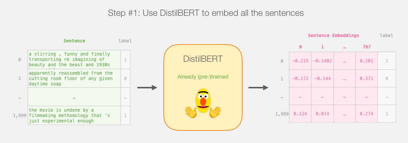
We will not touch distilBERT after this step. It’s all Scikit Learn from here. We do the usual train/test split on this dataset:

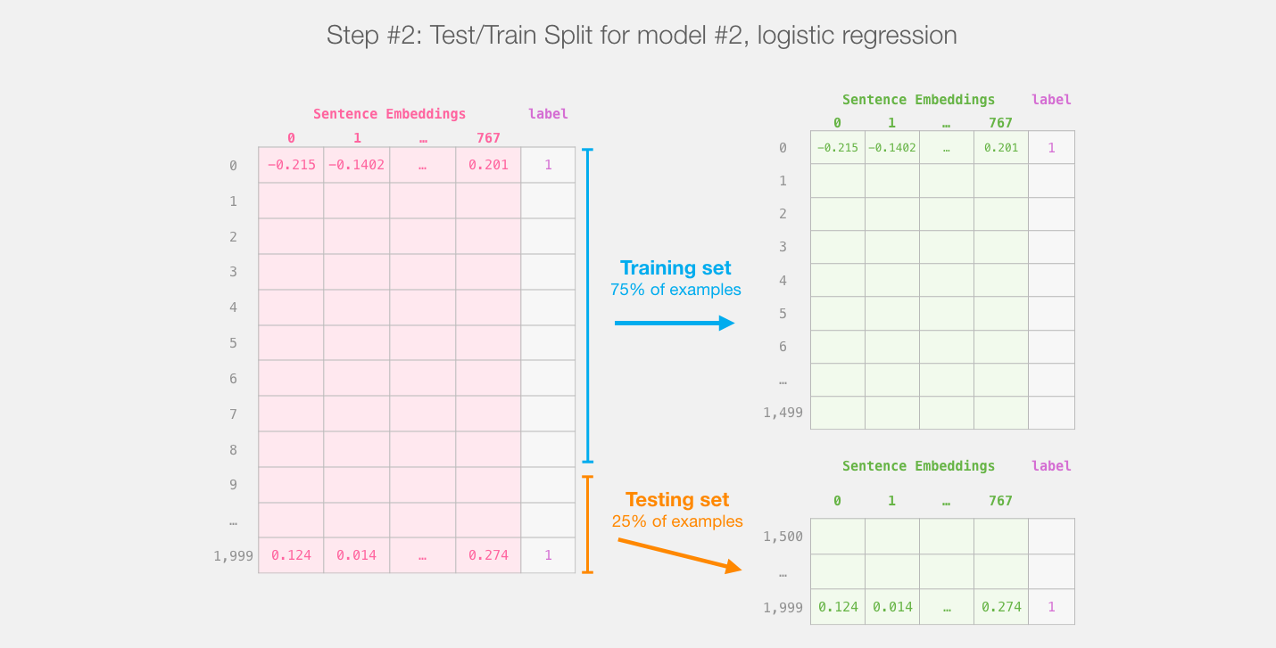
Train/test split for the output of distilBert (model #1) creates the dataset we'll train and evaluate logistic regression on (model #2). Note that in reality, sklearn's train/test split shuffles the examples before making the split, it doesn't just take the first 75% of examples as they appear in the dataset.

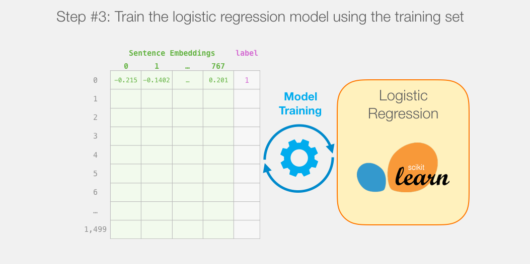
Then we train the logistic regression model on the training set:

How a single prediction is calculated

Before we dig into the code and explain how to train the model, let’s look at how a trained model calculates its prediction.

Let’s try to classify the sentence “a visually stunning rumination on love”. The first step is to use the BERT tokenizer to first split the word into tokens. Then, we add the special tokens needed for sentence classifications (these are [CLS] at the first position, and [SEP] at the end of the sentence).

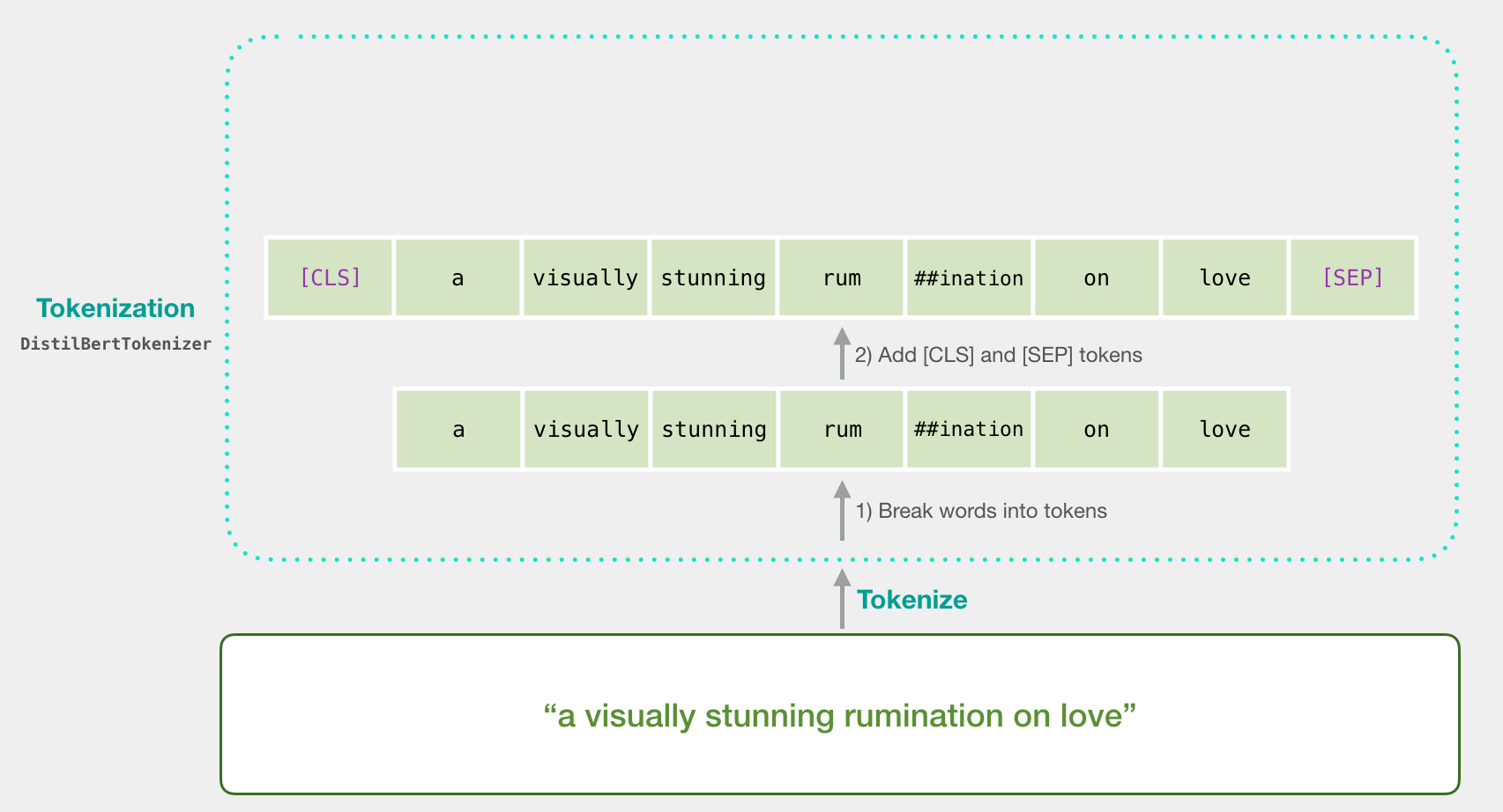
The third step the tokenizer does is to replace each token with its id from the embedding table which is a component we get with the trained model. Read The Illustrated Word2vec for a background on word embeddings.

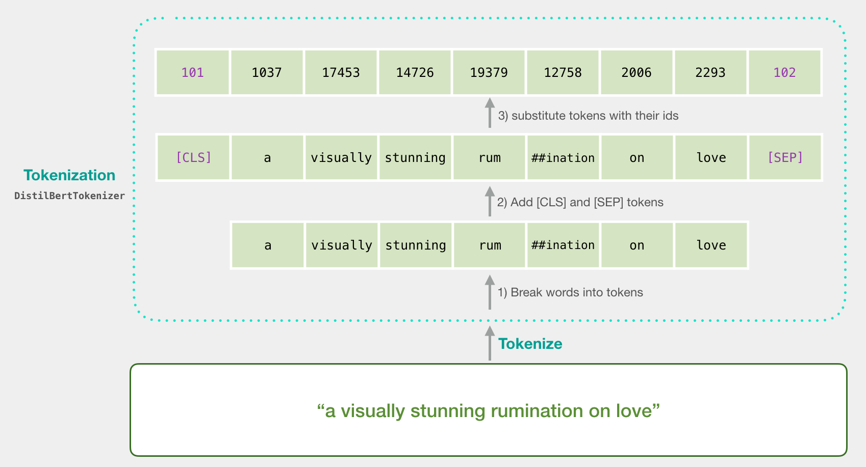
Note that the tokenizer does all these steps in a single line of code:

tokenizer.encode("a visually stunning rumination on love", add_special_tokens=True)

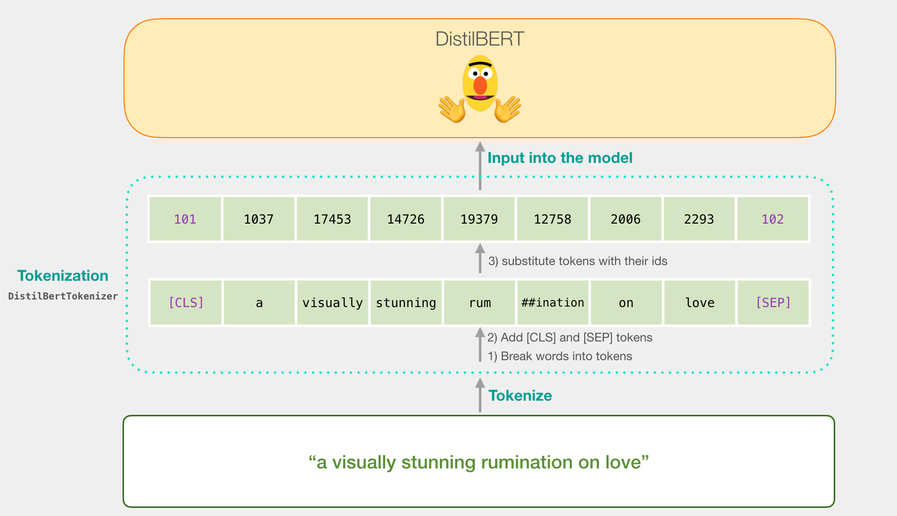
Our input sentence is now the proper shape to be passed to DistilBERT.

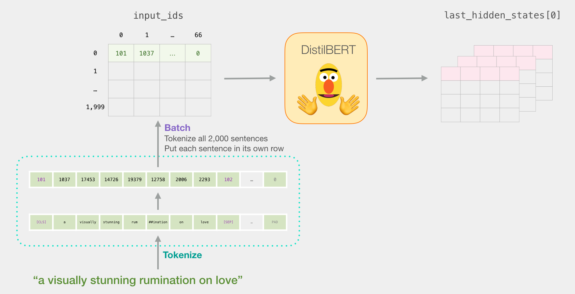
If you’ve read Illustrated BERT, this step can also be visualized in this manner:

Flowing Through DistilBERT

Passing the input vector through DistilBERT works just like BERT. The output would be a vector for each input token. each vector is made up of 768 numbers (floats).

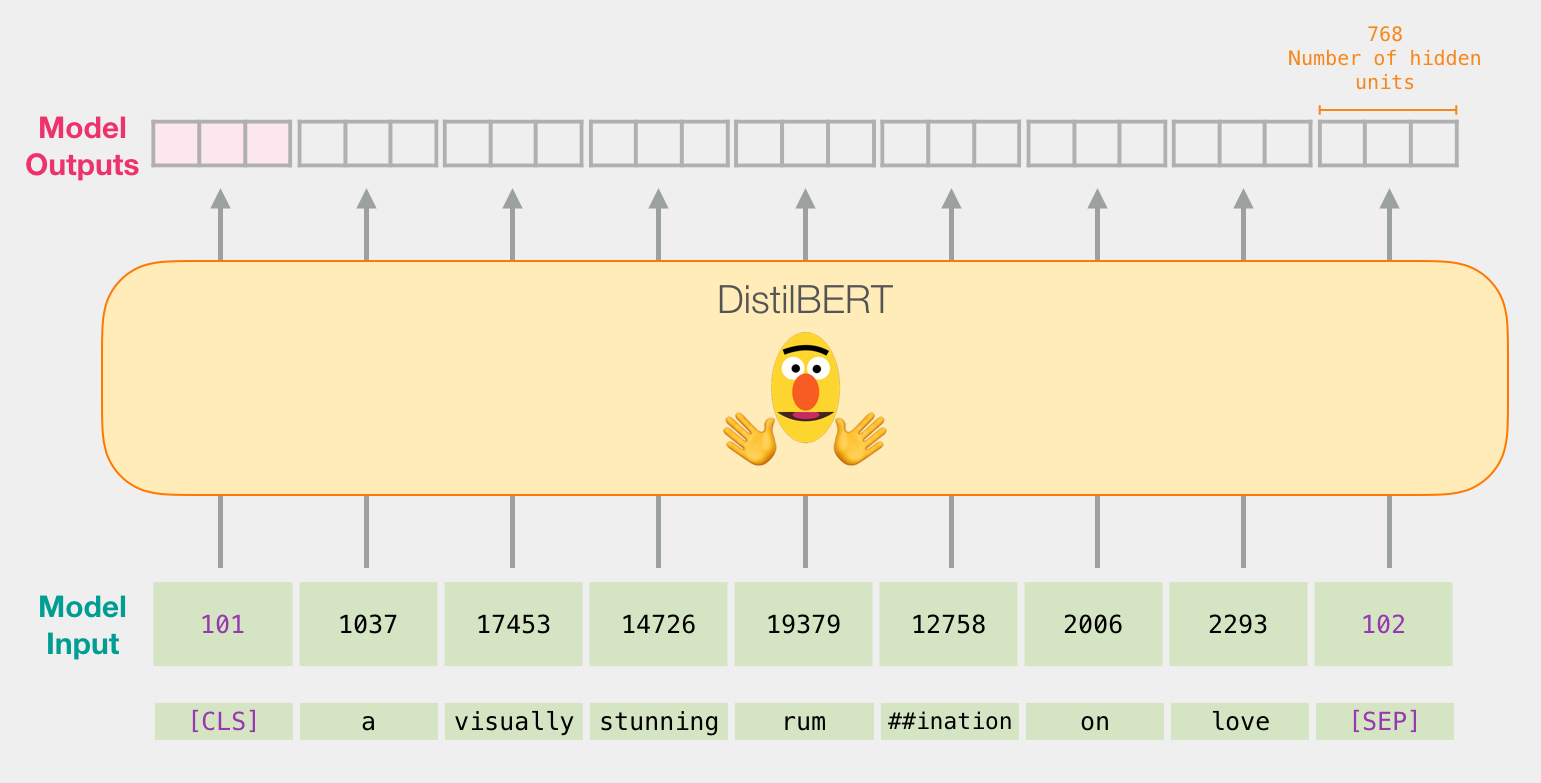
Because this is a sentence classification task, we ignore all except the first vector (the one associated with the [CLS] token). The one vector we pass as the input to the logistic regression model.

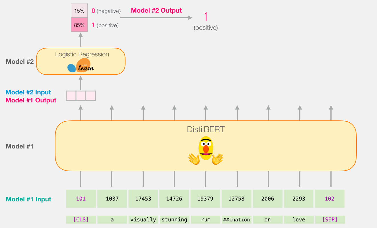
From here, it’s the logistic regression model’s job to classify this vector based on what it learned from its training phase. We can think of a prediction calculation as looking like this:

The training is what we’ll discuss in the next section, along with the code of the entire process.

The Code

In this section we’ll highlight the code to train this sentence classification model. A notebook containing all this code is available on colab
Let’s start by importing the tools of the trade

import numpy as np
import pandas as pd
import torch
import transformers as ppb # pytorch transformers
from sklearn.linear_model import LogisticRegression
from sklearn.model_selection import cross_val_score
from sklearn.model_selection import train_test_split

The dataset is available as a file on github, so we just import it directly into a pandas dataframe

df = pd.read_csv('https://github.com/clairett/pytorch-sentiment-classification/raw/master/data/SST2/train.tsv', delimiter='\t', header=None)

We can use df.head() to look at the first five rows of the dataframe to see how the data looks.

df.head()

Which outputs:

Importing pre-trained DistilBERT model and tokenizer

model_class, tokenizer_class, pretrained_weights = (ppb.DistilBertModel, ppb.DistilBertTokenizer, 'distilbert-base-uncased')

## Want BERT instead of distilBERT? Uncomment the following line:
#model_class, tokenizer_class, pretrained_weights = (ppb.BertModel, ppb.BertTokenizer, 'bert-base-uncased')

# Load pretrained model/tokenizer
tokenizer = tokenizer_class.from_pretrained(pretrained_weights)
model = model_class.from_pretrained(pretrained_weights)

We can now tokenize the dataset. Note that we’re going to do things a little differently here from the example above. The example above tokenized and processed only one sentence. Here, we’ll tokenize and process all sentences together as a batch (the notebook processes a smaller group of examples just for resource considerations, let’s say 2000 examples).

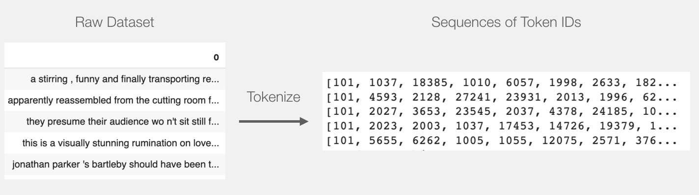
Tokenization

tokenized = df[0].apply((lambda x: tokenizer.encode(x, add_special_tokens=True)))

This turns every sentence into the list of ids.

The dataset is currently a list (or pandas Series/DataFrame) of lists. Before DistilBERT can process this as input, we’ll need to make all the vectors the same size by padding shorter sentences with the token id 0. You can refer to the notebook for the padding step, it’s basic python string and array manipulation.

After the padding, we have a matrix/tensor that is ready to be passed to BERT:

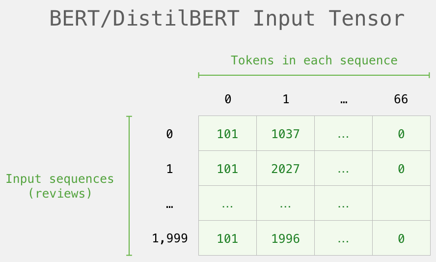
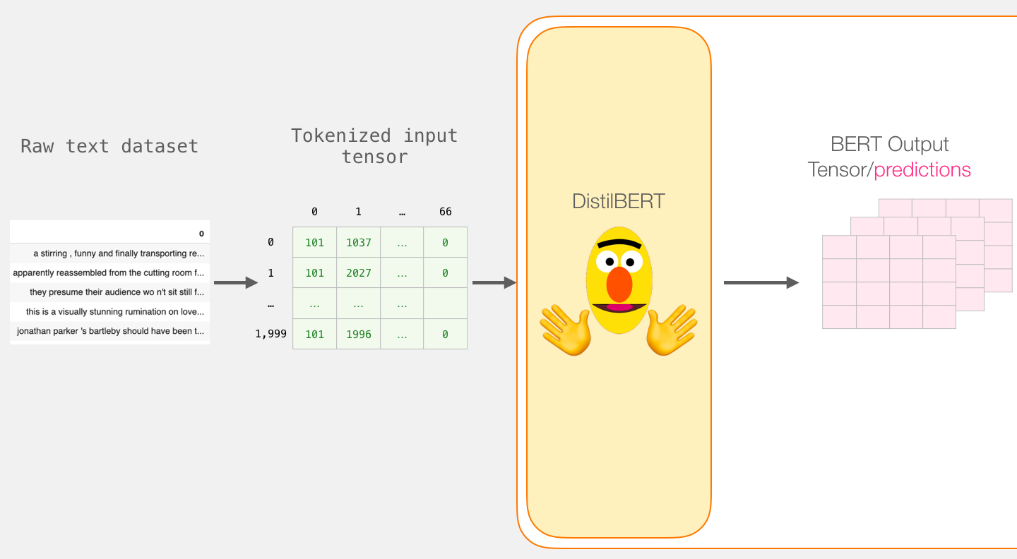
Processing with DistilBERT

We now create an input tensor out of the padded token matrix, and send that to DistilBERT

input_ids = torch.tensor(np.array(padded))
with torch.no_grad():
    last_hidden_states = model(input_ids)

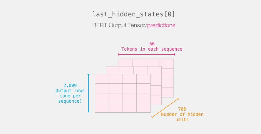
After running this step, last_hidden_states holds the outputs of DistilBERT. It is a tuple with the shape (number of examples, max number of tokens in the sequence, number of hidden units in the DistilBERT model). In our case, this will be 2000 (since we only limited ourselves to 2000 examples), 66 (which is the number of tokens in the longest sequence from the 2000 examples), 768 (the number of hidden units in the DistilBERT model).

Unpacking the BERT output tensor

Let’s unpack this 3-d output tensor. We can first start by examining its dimensions:

Recapping a sentence’s journey

Each row is associated with a sentence from our dataset. To recap the processing path of the first sentence, we can think of it as looking like this:

Slicing the important part

For sentence classification, we’re only only interested in BERT’s output for the [CLS] token, so we select that slice of the cube and discard everything else.

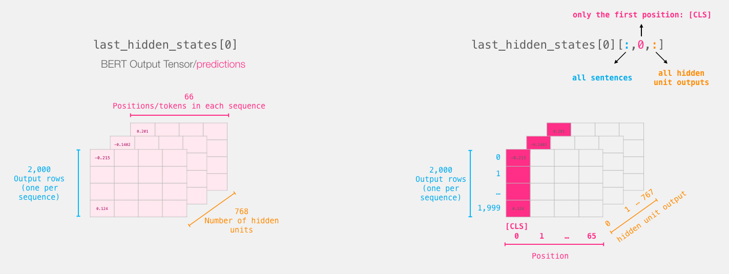
This is how we slice that 3d tensor to get the 2d tensor we’re interested in:

 # Slice the output for the first position for all the sequences, take all hidden unit outputs
features = last_hidden_states[0][:,0,:].numpy()

And now features is a 2d numpy array containing the sentence embeddings of all the sentences in our dataset.

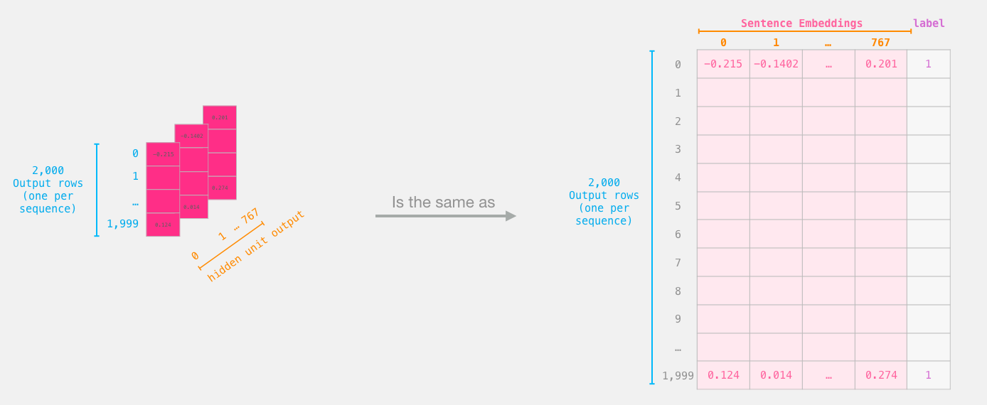
The tensor we sliced from BERT's output

Dataset for Logistic Regression

Now that we have the output of BERT, we have assembled the dataset we need to train our logistic regression model. The 768 columns are the features, and the labels we just get from our initial dataset.

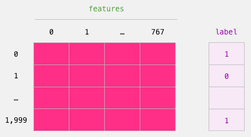
The labeled dataset we use to train the Logistic Regression. The features are the output vectors of BERT for the [CLS] token (position #0) that we sliced in the previous figure. Each row corresponds to a sentence in our dataset, each column corresponds to the output of a hidden unit from the feed-forward neural network at the top transformer block of the Bert/DistilBERT model.

After doing the traditional train/test split of machine learning, we can declare our Logistic Regression model and train it against the dataset.

labels = df[1]
train_features, test_features, train_labels, test_labels = train_test_split(features, labels)

Which splits the dataset into training/testing sets:

Next, we train the Logistic Regression model on the training set.

lr_clf = LogisticRegression()
lr_clf.fit(train_features, train_labels)

Now that the model is trained, we can score it against the test set:

lr_clf.score(test_features, test_labels)

Which shows the model achieves around 81% accuracy.