EEG PROCESSING GUI MANUAL - katielavigne/EEG_ProcessingGUI GitHub Wiki
Original version: 25/01/2016
IMPORTANT
- GUI will only work with MCT/OTT BADE, FISH, and WM tasks!
- Ensure data is in the proper directory structure before beginning!
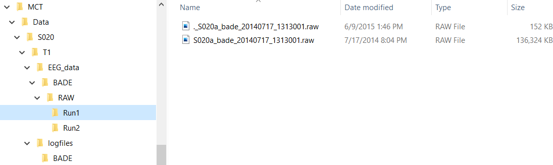
Data Organization
- Folders and filenames cannot contain spaces!
- Subject IDs in folders and filenames must be consistent (including case)!
- Each run folder should only have a single .raw file; in the case of .mat data, only a single file should be in the MAT folder.
- Data files must have the appropriate .raw/.mat extension
- The logfiles directory should only contain the relevant .log/.txt files, extra files from aborted runs should be moved. Consider creating a “BAD_DATA” folder (within the logfiles directory is fine) and move the bad .log/.txt files in there.
- Having the data properly organized will make things run much more smoothly!
1. OPEN GUI
- Open MATLAB and cd to the parent directory to your data/processing directories (e.g., if data directory is /data4/EEG/MCT/Data, cd to /data4/EEG/MCT)
Not required, but makes things easier when selecting directories
- Type in “runEEG” without quotes (note: both the EEGlab and EEGProcessingGUI folders (and subfolders) must be in your MATLAB path)
EEGlab is located under the MATLAB toolboxes directory (if not, download from http://sccn.ucsd.edu/eeglab/install.html)
- The EEGlab GUI will open – don’t close it.
- The EEG Processing GUI looks like this:
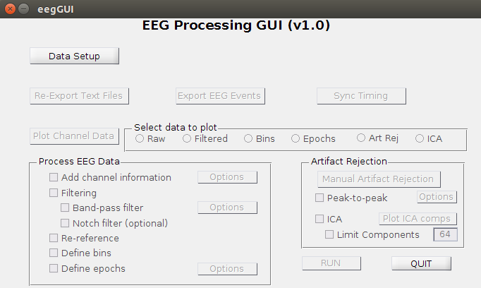
2. DATA SETUP
-
Click on Data Setup and a new window will pop up:

-
Select data directory (with all the subject folders)
-
Select processing directory (where data will be saved)
-
Wildcards: determine which subjects/sessions/tasks/runs to be processed (note: these are case-sensitive!)
Example: selects all subjects, all sessions, BADE only, and all runs under /data4/EEG/MCT/Data
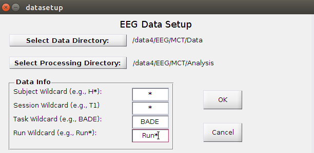
- Data Info Options
Subject Wildcard: * (all), A*/H*/S* (group), S100 (single subject)
Session Wildcard: * or T* (all), T1/T3 (single session)
Task Wildcard: * (all), BADE/FISH/WM (single task)
Run Wildcard: Run* (depends on folder names, but this is the standard)
- Click OK. The active buttons in the main window will change depending on the data selected and whether it can find the relevant files, etc. For unprocessed data, only the three buttons under Data Setup will be active. If already-processed data is found, other options will be active as well.
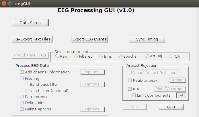
3. RE-EXPORT TEXT FILES
- Click Re-Export Text Files
- This step will re-export the .txt versions of the Presentation logfiles and add a “fixed” suffix to the filename (e.g., MCT_S101a_run1_eventTiming_bade_fixed.txt) into the relevant logfile directory.
This is necessary because the original text files that are automatically generated during testing do not include all events (e.g., non-final responses, start of run, etc.), and this causes issues when trying to sync the EEG and Presentation timing. Also, for FISH, the condition names in the text files are too long.
TO BE CHECKED: Linux is required because in some cases there was a conflict when sending the codes to the EEG computer, leading to missing events in the EEG files. This step will call a Linux script to find those missing codes and remove them from the re-exported text file (to be re-added later during the syncing step). This step will not fail if you are on a Windows OS, but if there are missing codes, this will lead to the Presentation timing being used in the syncing step, instead of the more accurate EEG timing.
- Any errors will be displayed in the Matlab command window, so be sure to check them before continuing. In the example below, all of these are acceptable errors, because the subjects either don’t have any data collected yet or they are not valid subjects/sessions. This occurs because we have extra folders in the data directory (pilot testing, T3 placeholders, etc). In cases where a conflict was found, the ‘OK!’ signifies that it has been removed and will be added back in later.
4. EXPORT EEG EVENTS
- Click Export EEG Events This step will export the EEG events from the .raw or .mat data files to text files. It will also create a subjinfo.csv file including the relevant subject information and filenames for the data files and logfiles to be used in the next step.
If the GUI can’t find the data file, or finds multiple data files in the relevant folder, it will prompt you to select the proper file.
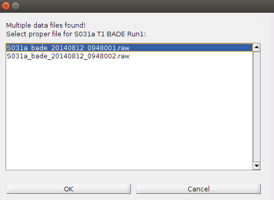
If the GUI can’t find the generic re-exported text file (e.g., MCT_S101a_run1_eventTiming_bade_fixed.txt) or finds multiple files, it will also prompt you to select the proper file (this should not happen if you re-exported the text files).
Note: make sure your data is organized properly (see page 1) to prevent this kind of user input!
- When complete, a pop-up will notify you if there were any errors. Errors will be saved in the user-defined processing directory under EEGevent_errors.txt. Check this file before proceeding to the next step!
5. SYNC TIMING
Excel SyncEEGTiming.xlsm Sheet
In order for the Sync Timing step to work, you will need to determine the start times of the EEG relative to Presentation, and add that time to the Presentation timing. Use the SyncEEGTiming.xlsm Excel sheet to find the corresponding timing.
Note: Use Microsoft Excel in Windows, macro not tested on other spreadsheet programs. TO BE CHECKED IF CAN INCORPORATE IN MATLAB.
-
Open SyncEEGTiming.xlsm and the subjinfo.csv file created in the previous step
-
Copy the contents of the subjinfo.csv sheet to the SubjInfo sheet in SyncEEGTiming.xlsm and close subjinfo.csv
-
Run the macro with Ctrl + T
-
Select data and trigger (processing directory/Triggers) directories corresponding to those in the EEG GUI
-
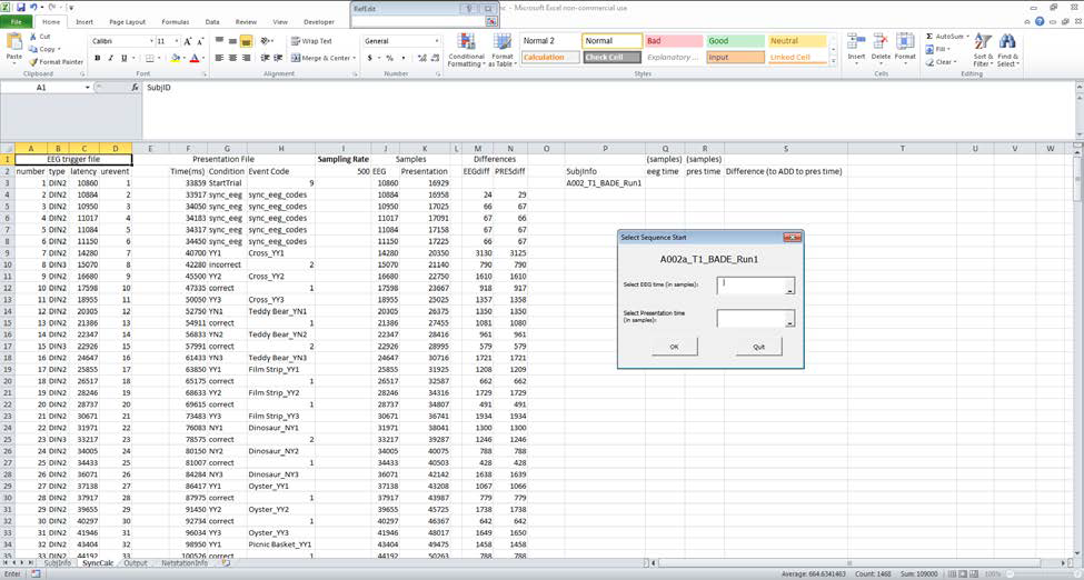
The macro will open the EEG trigger and Presentation .txt files and paste the relevant information into the SyncCalc sheet. A pop-up will ask you to select the timing (in samples) for the start of the sequence for both EEG timing (column J) and Presentation timing (column K).
-
Use the differences columns (M & N) to find a sequence of events that match. These columns show the differences between adjacent events (one per each row). By examining the differences between events for both EEG and Presentation timing, you can see which events match up. It’s important to look for a sequence of ~5 events matching so that you can be sure the events are aligned and not just randomly showing the same difference.
-
Start from after the sync_eeg_codes events (in this example, the run starts at N9), and go down comparing columns M and N to see if the differences match up (don’t worry if they are a few samples off)
-
In this example, they match up quite well (which is the case with newer data), with the exception of an extra DIN event (DIN4), which is to be expected with UBC data. Find the start of the sequence for both EEG (M10) and Presentation (N9) and select the corresponding cells in the Samples columns (in this case, J10 and K9). Then click OK.
-
Clicking OK with empty values in one or both fields will skip the subject (do this if you can’t find a sequence and think you may have chosen the wrong data/logfile in the Export EEG Events step).
-
Clicking OK with a range of cells selected in one or both fields will prompt a warning and you will be asked to redo the subject.
-
Clicking QUIT will stop the macro. When you re-run the macro again, it will start where it left off.
-
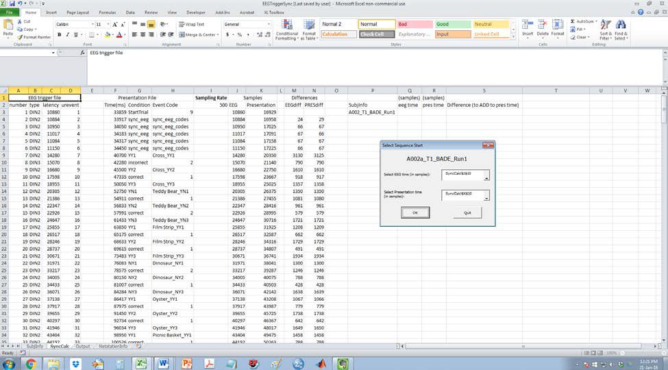
Rows P to S in the SyncCalc sheet will be populated with the times you selected and the difference between the two.
-
The Output sheet will be populated with all the relevant info needed for the EEG GUI’s Sync Timing step. This will be saved as a text file (syncinfo.txt) in the Trigger directory.Note. This file will be overwritten if it already exists!
Sync Timing (GUI)
- Note: This script creates a “ProcessedData” folder under the user-defined processing directory. Do not rename or remove it!
- This step will sync the EEG and Presentation timing based on the syncinfo.txt file created in the previous step, and will determine whether to use the Presentation timing or the more accurate EEG timing to list the events. The type of timing chosen depends on several factors, but in general it requires that the number of EEG events and Presentation events match up.
- Click Sync Timing on the GUI
- There should be no pop-ups until the syncing is complete, when it will let you know if there are any errors.
- Errors are saved to sync_errors.txt in the user-defined processing directory. Examine this file to see if the less accurate Presentation timing was used for any subjects. If so, there will be a line saying “[Subject] [Session] [Task]: # extra DINs/Presentation events found, presentation time used!”
This should not happen for most participants. Many internal checks are included in the GUI, so the events should match up in most cases.
- If there is a syncing error, you can look at the “_timecomp.txt” file in the relevant subject processing folder to see which events don’t match up, and the “_event_latencies.txt” file to see the differences between the EEG and Presentation events (note: the event latencies file is not perfect, so it’s more for a general idea). You can then decide if the latencies are acceptable or if you want to try to fix the events by possibly removing the extra ones and syncing again.
- This step will output a “*sync_all.txt” file in the relevant logfile sub-directory for each subject/session/task, which includes the final timing (either EEG timing or presentation depending on if the number of events matched), and the Presentation condition and event codes for all runs combined.
- The combined and synced data will also be saved as “*_raw.set/.fdt” files in the relevant processing sub-directory, which is what is used in the processing steps.
6. CHECK TIMING SYNC
- Click on “Raw” under “Select data to plot” and click “Plot Channel Data”
- Select display options or use defaults
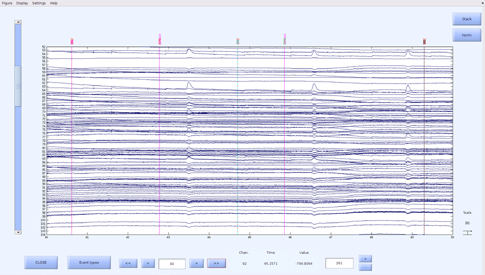
- A figure with the title “Scroll channel activities – [.set filename]” will open
- You can change the display options in the figure as well
- Scroll through to make sure all events are synced up
The events should be identical if EEG timing was used, unless there were missing codes, in which case those will not be synced to an event
- If Presentation timing was used, you can use this figure to find which events are not matching
- Click Close in bottom right when finished
- A pop-up will allow you to go directly to the next subject or quit
- Example of a good synchronization:
7. PROCESSING
These steps can be done either one at a time or altogether. New .set/.fdt files will be created at each step. These can be deleted afterwards if desired (e.g., find [parent path] –name “_chaninfo.” –delete)
- Click on the checkbox next to the step to activate the processing step and select options if applicable
The options buttons are the same as the pop-ups when clicking on the checkboxes; use these if you want to modify an option after selecting it (or simply deselect and select)
- Default options are listed for all steps, but may want/need to be changed.
Add channel information
- Navigate to and select the sfp file which contains channel information (e.g., GSN256_noFid.sfp)
- List channels (1: # channels) and reference electrode (e.g., Cz)
- Click OK.
- Click Run or select next step.
- Will save “*_chaninfo. set/.fdt” files
Filtering
- When activated, the bandpass filter options will pop-up. You can also select notch if desired
Band-pass filter: type in desired filter type (e.g., butter) and frequency values for high pass (e.g., 0.05) and low pass (e.g., 100) filters
Notch filter (optional): no options (default is 60Hz).
- Click OK
- Click Run or select next step.
- Will save “*_filt. set/.fdt” files
Re-reference
- There are no options for this step.
- Click Run or select next step.
- Will save “*_filt_reref. set/.fdt” files
Define bins
- There are no options for this step, but make sure the two text files under EEGProcessingGUI/binfiles ([Task]_eventTypes.txt and [Task]_bdf.txt) are accurate before continuing.
- Click Run or select next step.
- Will save “*_filt_reref_bins. set/.fdt” files
Define epochs
- Enter epoch range (e.g., -500 4000) with a space in between the lower and upper bounds Default is 10,000 right now TO BE CHECKED
- Click Run.
- Will save “*_epochs. set/.fdt” files
Note: EEGlab writes a lot of information to the command window, which can go by quickly and get lost when running multiple subjects. This output is now saved for each subject/session/task to the relevant processing sub-directories under “processinginfo_[date].txt”, and can be examined if there are any issues during processing. Any subsequent processing run on the same date will be appended to this file, unless “add channel information” is selected, in which case, it will delete and create a new file. This is to avoid confusion when re-running the data multiple times, but still allow for changes in intermediate steps to be recorded. Each new processing “run” will start with the date and time and several asterisks above it to show a new section.
8. ARTIFACT REJECTION
Manual Artifact Rejection
- Click on the “Manual Artifact Rejection” button
- Select window length and number of channels to display (this can be modified during as well)
- See section 9.1.2. of EEG Analysis Protocol for rejection guidelines
- Select all the epochs you want to reject and click Reject in the bottom right-hand corner
- Click Yes
- The file will be saved the file as “*_epochs_artrejman.set”. If you don’t reject any epochs, it will still be saved under the new name.
- Select Next Subject or Quit.
Peak-to-Peak Artifact Rejection (not recommended)
- Click on “Peak-to-Peak”
- See section 9.1.1 if EEG Analysis Protocol for option guidelines
- Click Run
- The script will first look for any manually-rejected data “_epochs_artrejman.set” and if not found, will load the “_epochs.set” data
- It will add the suffix “_p2p” to whatever file it loaded (e.g., “*_epochs_artrejman_p2p.set”)
9. ICA
- Click on “ICA”
- Click on “Limit Components” if you want to do PCA and type in the number of components
- Click Run
- The script will first look for a file in which ICA components have already been removed (in case you want to remove more components after already doing so): “*_ICApruned.set”.
- If not found, it will find all the “epochs.set” files and if there is only one, will run ICA on that. Otherwise, it will ask you to select the file you want to run ICA on.
This is useful if you’ve run multiple artifact rejection techniques and only want to select one.
Because it searches for “epochs.set”, you will not be able to run the ICA without artifact rejection (either manual or peak to peak). If you do not want to reject any epochs, simply open Manual Artifact Rejection, and close without rejecting.
10. Plot ICA Components
- Click on “Plot ICA Comps”
- Select the range of components you wish to plot (e.g., 1:64)
- Click OK
- See section 9.1.3 of EEG Analysis Protocol for guidelines on rejecting ICA components
- New ICA-rejected data will be saved as “*_ICApruned.set”
- Select Next Subject or Quit.