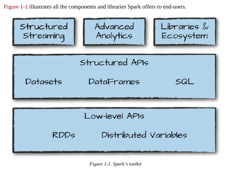
Apache Spark is a unified computing engine and a set of libraries for parallel data processing on computer clusters.

At the same time that Spark strives for unification, it carefully limits its scope to a computing engine. By this, we mean that Spark handles loading data from storage systems and performing computation on it, not permanent storage as the end itself. You can use Spark with a wide variety of persistent storage systems, including cloud storage systems such as Azure Storage and Amazon S3, distributed file systems such as Apache Hadoop, key-value stores such as Apache Cassandra, and message buses such as Apache Kafka. However, Spark neither stores data long term itself, nor favors one over another. The key motivation here is that most data already resides in a mix of storage systems. Data is expensive to move so Spark focuses on performing computations over the data, no matter where it resides.

. Now, a group of machines alone is not powerful, you need a framework to coordinate work across them. Spark does just that, managing and coordinating the execution of tasks on data across a cluster of computers. The cluster of machines that Spark will use to execute tasks is managed by a cluster manager like Spark’s standalone cluster manager, YARN, or Mesos. We then submit Spark Applications to these cluster managers, which will grant resources to our application so that we can complete our work.

Spark Applications

Spark Applications consist of a driver process and a set of executor processes. The driver process runs your main() function, sits on a node in the cluster, and is responsible for three things: maintaining information about the Spark Application; responding to a user’s program or input; and analyzing, distributing, and scheduling work across the executors (discussed momentarily). The driver process is absolutely essential—it’s the heart of a Spark Application and maintains all relevant information during the lifetime of the application.

The executors are responsible for actually carrying out the work that the driver assigns them. This means that each executor is responsible for only two things: executing code assigned to it by the driver, and reporting the state of the computation on that executor back to the driver node.

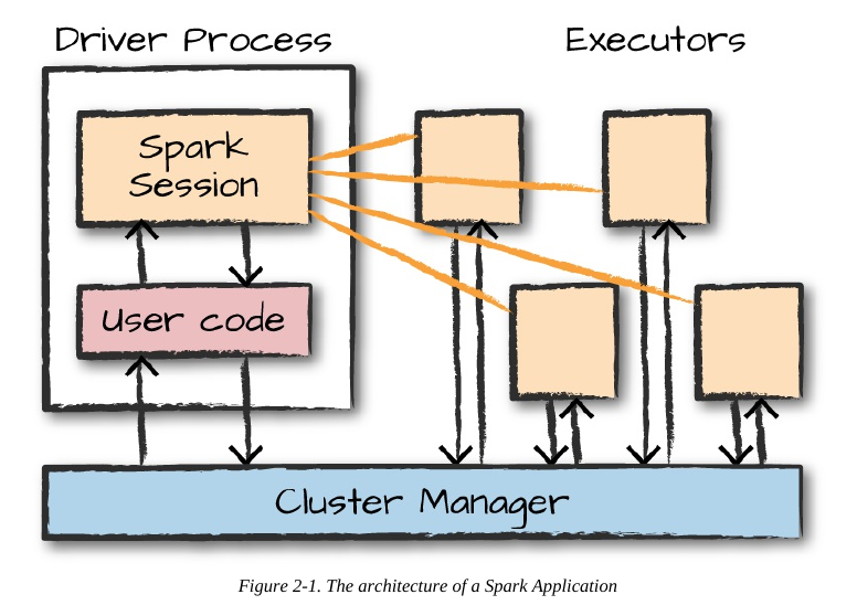
In this diagram, we removed the concept of cluster nodes. The user can specify how many executors should fall on each node through configurations.

Here are the key points to understand about Spark Applications at this point: Spark employs a cluster manager that keeps track of the resources available. The driver process is responsible for executing the driver program’s commands across the executors to complete a given task. The executors, for the most part, will always be running Spark code. However, the driver can be “driven” from a number of different languages through Spark’s language APIs. Let’s take a look at those in the next section.

The SparkSession

As discussed in the beginning of this chapter, you control your Spark Application through a driver process called the SparkSession. The SparkSession instance is the way Spark executes user-defined manipulations across the cluster.

You can think of a DataFrame as a spreadsheet with named columns. Figure 2-3 illustrates the fundamental difference: a spreadsheet sits on one computer in one specific location, whereas a Spark DataFrame can span thousands of computers.

If you have one partition, Spark will have a parallelism of only one, even if you have thousands of executors. If you have many partitions but only one executor, Spark will still have a parallelism of only one because there is only one computation resource.

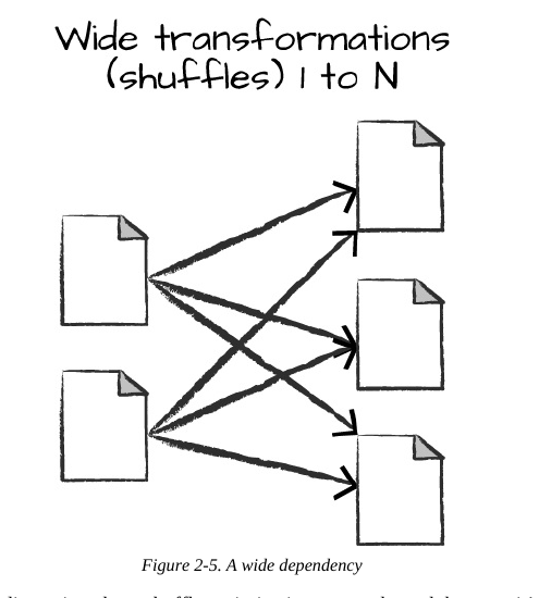
Narrow Vs Wide Transformations

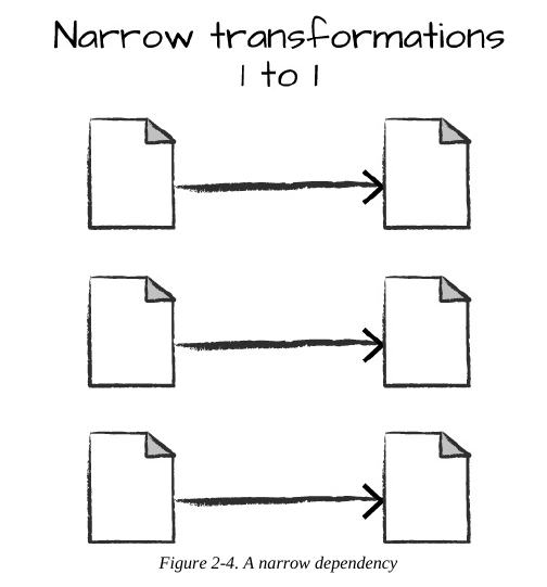
Transformations consisting of narrow dependencies (we’ll call them narrow transformations) are those for which each input partition will contribute to only one output partition.

A wide dependency (or wide transformation) style transformation will have input partitions contributing to many output partitions. You will often hear this referred to as a shuffle whereby Spark will exchange partitions across the cluster. With narrow transformations, Spark will automatically perform an operation called pipelining, meaning that if we specify multiple filters on DataFrames, they’ll all be performed in-memory. The same cannot be said for shuffles. When we perform a shuffle, Spark writes the results to disk. Wide transformations are illustrated in

n. By default, when we perform a shuffle, Spark outputs 200 shuffle partitions. Let’s set this value to 5 to reduce the number of the output partitions from the shuffle: spark.conf.set("spark.sql.shuffle.partitions", "5") flightData2015.sort("count").take(2)

With Spark SQL, you can register any DataFrame as a table or

view (a temporary table) and query it using pure SQL. There is no performance difference between writing SQL queries or writing DataFrame code, they both “compile” to the same underlying plan that we specify in DataFrame code.

You can make any DataFrame into a table or view with one simple method call:

flightData2015.createOrReplaceTempView("flight_data_2015")
// in Scala
val sqlWay = spark.sql("""
SELECT DEST_COUNTRY_NAME, count(1)
FROM flight_data_2015
GROUP BY DEST_COUNTRY_NAME
""")
val dataFrameWay = flightData2015
.groupBy('DEST_COUNTRY_NAME)
.count()
sqlWay.explain
dataFrameWay.explain
# in Python
sqlWay = spark.sql("""
SELECT DEST_COUNTRY_NAME, count(1)
FROM flight_data_2015
GROUP BY DEST_COUNTRY_NAME
""")
dataFrameWay = flightData2015\
.groupBy("DEST_COUNTRY_NAME")\
.count()
sqlWay.explain()
dataFrameWay.explain()

We will use the max function, to establish the maximum number of flights to and from any
given location. This just scans each value in the relevant column in the DataFrame and checks
whether it’s greater than the previous values that have been seen. This is a transformation,
because we are effectively filtering down to one row. Let’s see what that looks like:
spark.sql("SELECT max(count) from flight_data_2015").take(1)
// in Scala
import org.apache.spark.sql.functions.max
flightData2015.select(max("count")).take(1)
# in Python
from pyspark.sql.functions import max
flightData2015.select(max("count")).take(1)
Great, that’s a simple example that gives a result of 370,002. Let’s perform something a bit more
complicated and find the top five destination countries in the data. This is our first multi-
transformation query, so we’ll take it step by step. Let’s begin with a fairly straightforward SQL
aggregation:
// in Scala
val maxSql = spark.sql("""
SELECT DEST_COUNTRY_NAME, sum(count) as destination_total
FROM flight_data_2015
GROUP BY DEST_COUNTRY_NAME
ORDER BY sum(count) DESC
LIMIT 5
""")
maxSql.show()
# in Python
maxSql = spark.sql("""
SELECT DEST_COUNTRY_NAME, sum(count) as destination_total
FROM flight_data_2015
GROUP BY DEST_COUNTRY_NAME
ORDER BY sum(count) DESC
LIMIT 5
""")
maxSql.show()
+-----------------+-----------------+
|DEST_COUNTRY_NAME|destination_total|
+-----------------+-----------------+
|
 United States|
 411352|
|
 Canada|
 8399|
|
 Mexico|
 7140|
|
 United Kingdom|
 2025|
|
 Japan|
 1548|
+-----------------+-----------------+
Now, let’s move to the DataFrame syntax that is semantically similar but slightly different in
implementation and ordering. But, as we mentioned, the underlying plans for both of them are
the same. Let’s run the queries and see their results as a sanity check:
// in Scala
import org.apache.spark.sql.functions.desc
flightData2015
.groupBy("DEST_COUNTRY_NAME")
.sum("count")
.withColumnRenamed("sum(count)",.sort(desc("destination_total"))
.limit(5)
.show()
"destination_total")
# in Python
from pyspark.sql.functions import desc
flightData2015\
.groupBy("DEST_COUNTRY_NAME")\
.sum("count")\
.withColumnRenamed("sum(count)", "destination_total")\
.sort(desc("destination_total"))\
.limit(5)\
.show()
+-----------------+-----------------+
|DEST_COUNTRY_NAME|destination_total|
+-----------------+-----------------+
|
 United States|
 411352|
|
 Canada|
 8399|
|
 Mexico|
 7140|
|
 United Kingdom|
 2025|
|
 Japan|
 1548|
+-----------------+-----------------+
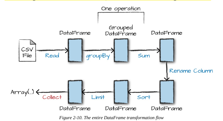
Now there are seven steps that take us all the way back to the source data. You can see this in the
explain plan on those DataFrames. Figure 2-10 shows the set of steps that we perform in “code.”
The true execution plan (the one visible in explain) will differ from that shown in Figure 2-10
because of optimizations in the physical execution; however, the llustration is as good of a
starting point as any. This execution plan is a directed acyclic graph (DAG) of transformations,
each resulting in a new immutable DataFrame, on which we call an action to generate a result.