Meso scale simulation of dry pore collapse - isale-code/isale-wiki GitHub Wiki
The example simulates the impact of a quartzite flyer plate hitting a quartzite target at 2000 m/s consisting of a sample with resolved pores. The sample is embedded in two buffer plates.
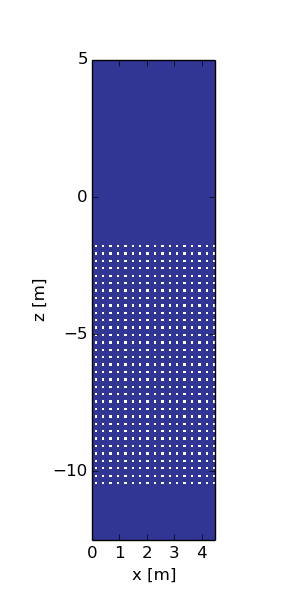
The model setup is very similar to a typical laboratory shock experiment. The impactor is a flyer plate which hits a buffer plate. The generated shock wave then travels through a sample which consists of resolved pores. The setup of the pores is defined by the user and the needed parameters are set in the asteroid input file.The default setup creates a mesh of regularly distributed squared pores each resolved by 8x8 cells, a total of about 500 pores in the sample. We suggest a hydrodynamic simulation. The pores are empty. If the distribution, porosity or number of pores needs to be changed the parameters for the pore space geometry in the asteroid.inp file as listed below need to be adjusted. You might want to adapt the size of the grid in asteroid.inp as well to ensure an even distribution of pores at the grid boundaries (left and right).
Go to the relevant example directory
cd /share/examples/mesoscale2D
Run iSALE2D. The simulation will take up to several hours, so this should be run in the background.
./iSALE2D &
Once the model has finished running, go into the model output directory and visualise the results by plotting pressure profiles or the pressure field.
Use pySALEPlot to produce profiles of the pressure pulse as it propagates through the mesh.
python Plotting/profiles.py
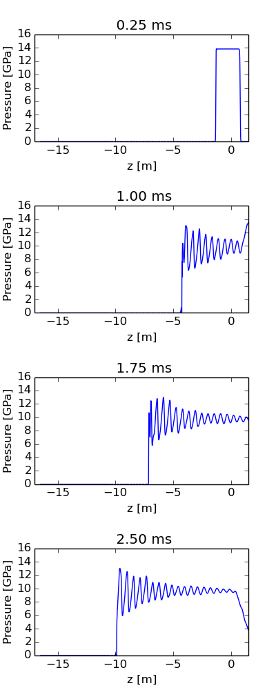
The image of the pressure profiles will be output to the Plots/ directory (as PreProfiles.png). These should be identical to those shown below.
You can also visulalise the propagation of the shock wave through the mesh step by step by using pySALEPlot.
python Plotting/Pre.py
You can see the images in the Plots/ directory.
The pySALEPlot plotting scripts (see also /share/examples/mesoscale2D/Plotting/Pre.py) can easily be modified to generate additional images or can be adapted to your specific problem.
Simulation setup is written in asteroid.inp:
------------------- General Model Info ---------------------------------
VERSION               __DO NOT MODIFY__             : 4.1
DIMENSION             dimension of input file       : 2
PATH                  Data file path                : ./
MODEL                 Modelname                     : mesoscale2D
A mesh geometry with a cell size of 1.5 cm:
------------------- Mesh Geometry Parameters ---------------------------
GRIDH               horizontal cells                : 0    :  325  :  0
GRIDV               vertical cells                  : 0    : 1730  :  20
GRIDEXT               ext. factor                   : 1.02d0
GRIDSPC               grid spacing                  : 1.5D-2
CYL                   cylinder symmetry             : 0.D0
The set-up type is @MESO_PORE@ with no gravity field.
------------------- Global Setup Parameters ----------------------------
S_TYPE                setup type                    : MESO_PORE
ALE_MODE              ALE modus                     : EULER
GRAD_TYPE             gradient type                 : NONE
A single impactor object strikes a one layer target. The quarzit impactor has a PLATE geometry (extending the full width of the mesh) with a half-thickness of 300 cells.
The impactor velocity is 2.0 km/s vertically down. The target layer extends from cell 1 to cell 1100.
The layer type is set to 20 relating to the mesoscale setup routine.
------------------- Projectile Parameters ------------------------------
OBJNUM                number of proj.               : 1
PR_TRACE              collision tracers             : 0
OBJRESH               CPPR horizontal               : 300
OBJVEL                object velocity               : -2.D3
OBJMAT                object material               : quarzit
OBJTYPE               object type                   : PLATE
------------------- Target Parameters ----------------------------------
LAYNUM                number of layers              : 1
LAYTYPE               layer type                    : 20
LAYPOS                layer position                : 1100
LAYMAT                layer material                : quarzit
The simulation duration is 5 milliseconds, with output saved every 50 microseconds.
------------------- Time Parameters ------------------------------------
TEND                  end time                      : 5.D-3
DTSAVE                save interval                 : 5.D-5
Deactivate the deviatoric stress model.
------------------- Control parameters (global) ------------------------
STRESS                Consider stress               : 0
A strengthless quartzite material model is used, with ANEOS-derived EoS tables.
-----------------------------------------------------------
MATNAME    Material name          : quarzit
EOSNAME    EOS name               : quarzit
EOSTYPE    EOS type               : aneos
STRMOD     Strength model         : HYDRO
DAMMOD     Damage model           : NONE
ACFL       Acoustic fluidisation  : NONE
PORMOD     Porosity model         : NONE
THSOFT     Thermal softening      : NONE
LDWEAK     Low density weakening  : NONE
--------------------------------------------------------
POIS       pois                   : 5.0000D-01
CHEAT      C_heat                 : 1.0000D+03
h2. How to setup a mesoscale simulation
The geometry has to defined in iSALE. Thus, we need to tell iSALE that we want to perform mesoscale simulations:
LAY_TYPE Layer type : 20
By doing so, iSALE will switch from the default setup-procedure to a separate setup-routine specifically designed for mesoscale problems (pore collapse). This routine requires additional parameters which need to be provided in a section within the asteroid input-file (asteroid.inp):
| abbreviation | Description | type | optional? | default value (if optional) |
|---|---|---|---|---|
| S_PORES | pore setup | integer | yes | 1 (regular distribution) |
| SAMPLE_T | sample area top | integer | yes | top of buffer plate-100cells |
| SAMPLE_B | sample area bottom | integer | yes | 400 |
| P_WIDTH | pore width | integer | yes | 8 |
| P_HEIGHT | pore height | integer | yes | 8 |
| PORE_XD | pore distance (X) | integer | yes | 10 |
| PORE_YD | pore distance (Y) | integer | yes | 10 |
| POROSITY | porosity | double | yes | 20 |
| PORE_max | max. pore size | integer | yes | 20 |
| PORE_T | pore type | integer | yes | 1 (squares) |
| PORE_N | number of ind. pores | integer | yes | 1 |
| P_LC_X | start pore in x | integer | yes | 1 (first cell) |
| P_LC_Y | start pore in y | integer | yes | 1 (first cell) |
These parameters can be used to define the arrangement and number of pores in the sample.
The setup of pores or the arrangement of pores is defined by
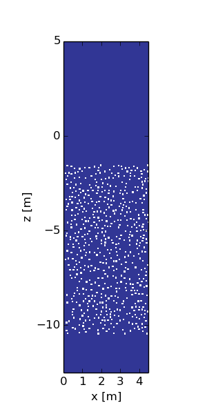
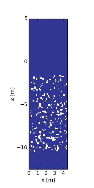
S_PORES setup pores : 1The possible setups are: 1 = pores regular, 2 = randomly distributed, 3 = random pores (size,distribution, overlapping), 4 = individual pores
To define the area where the sample with resolved pore is located within the target:
SAMPLE_T sample area top      : 1000
SAMPLE_B sample area bottom   :  400
The sample starts on top of a buffer plate and ends usually 100 cells below the flyer plate (leaving a buffer plate between flyer plate and sample). These parameters are neglected if S_PORES is set to 4 (individual pores).
The pore type, the dimensions of each pore (in cells) and the distance between the pores is defined by:
PORE_T   pore type            :    1
P_WIDTH  pore width           :    8
P_HEIGHT  pore height         :    8
PORE_XD  pore distance (X)    :   10
PORE_YD  pore distance (Y)    :   10
Available pore types are: 1=square, 2 = circle, 3= rhombus
In case of S_PORES = 4, the pore type and the dimension of each pore has to be defined individually and the distances are neglected in this case.
In case of random distribution of pores (S_PORES = 2,3), the porosity is defined by:
POROSITY     porosity         :   20.0d0
PORE_max    max. pore size    :   20
for S_TYPE=3 it is also required to define a maximum pore size.
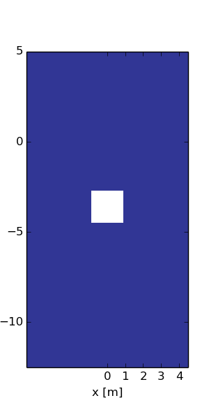
To set up individual pores (S_PORES=4), the number of the pores and the location of each pore (left corner of pore in x and y direction) has to be defined by:
PORE_N   num of ind. pores    : 1
P_LC_X start pore in x        : 1
P_LC_Y start pore in y        : 500
In case of more than one pore, list the values for each pore in columns separated by a colon.
The material of the matrix surrounding the open pore space is (as usual) defined in the line
LAY_MAT layer material : quarzit
Following points you may reconsider while setting up YOUR mesoscale model: If only one single pore is created make sure to set the P_LC_X to 1 to place the pore on the symmetry axis. If you use only single pores, you may want to adapt the total mesh size. If you like to change the porosity in the case of a regular distribution, change the pore dimension and the distance of pores. For a random distribution of pores, the initial porosity is read in by the additional parameters in asteroid.inp.
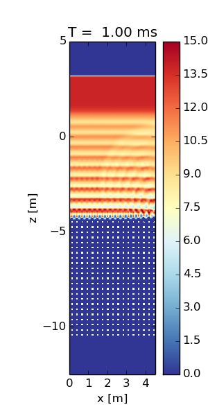
The figures below show the pressure along a vertical profile at several time steps after the initial impact. The initial pressure is about 14 GPa. Firstly, the shock wave propagates into the target quartzite (buffer plate) and the quartzite impactor. Then the shock wave reaches the first row of pore in the mesh resulting in the shown oscillations. The amplitude of the oscillations differ depending on location of the shock wave in relation to open pore space.
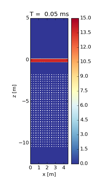
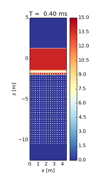
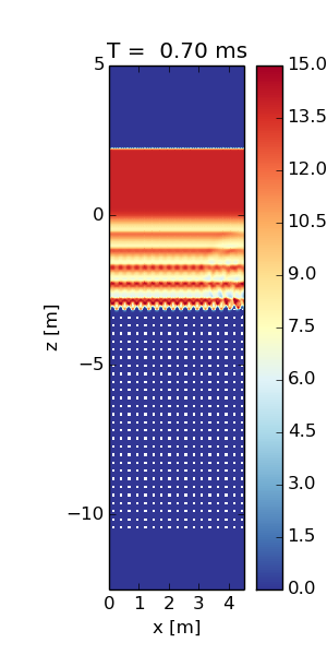
The following figures show the pressure field at several time steps as the shock wave propagates through the sample with resolved pores.
 |
 |
|---|---|
 |
 |
Here we provide some sketches of different possible setups:
- regular distribution
- random distribution
- random distribution with different pore sizes and possible overlapping
- one individual pore
| regular | random | random 2 | single pore |
|---|---|---|---|
 |
 |
 |
 |
