Airburst - isale-code/isale-wiki GitHub Wiki

The model is a low-resolution model of a 1kT (TNT energy equivalent) airburst at 100m altitude. The air is represented by a material model with an ideal gas equation of state (using a simplified Tillotson model) and an inviscid constitutive model. The Tillotson EoS is reduced to the ideal gas equation by setting all Tillotson parameters to zero, except the density at reference pressure (TL_RHO0), the specific heat capacity (TL_CHEAT) and a Tillotson parameter that reduces to the Grüneisen parameter for an ideal gas (TL_THERMA). In the case of an ideal gas, iSALE interprets the specific heat capacity as the specific gas constant Rs. The simulation ends after 3.8 s when the shock wave nearly has reached the lateral boundary.

The example demonstrates how to set-up iSALE2D for problems involving the static release of energy instead of a kinetic impactor. It also demonstrates the use of "probes" to record the state of parcels of material or places in the mesh at every tilmestep during the simulation.

Go to the relevant example directory

cd /share/examples/Airburst

Run iSALE2D. The simulation will take several hours, so this should be run in the background.

./iSALE2D &

From this directory you can produce images of the simulation to visualise the expansion and decay of the shock wave. First you call

python Plotting/blast_decay.py 

to extract the data from the “PROBES”-file in the Airburst example directory. The probe array is defined in the asteroid input file. Then call

python Plotting/pressure_snapshots.py

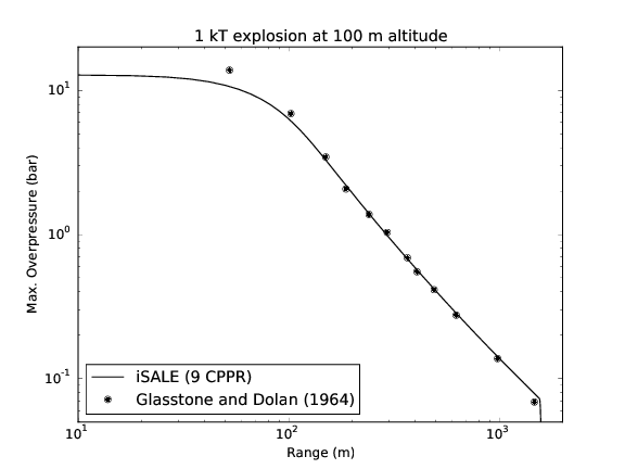
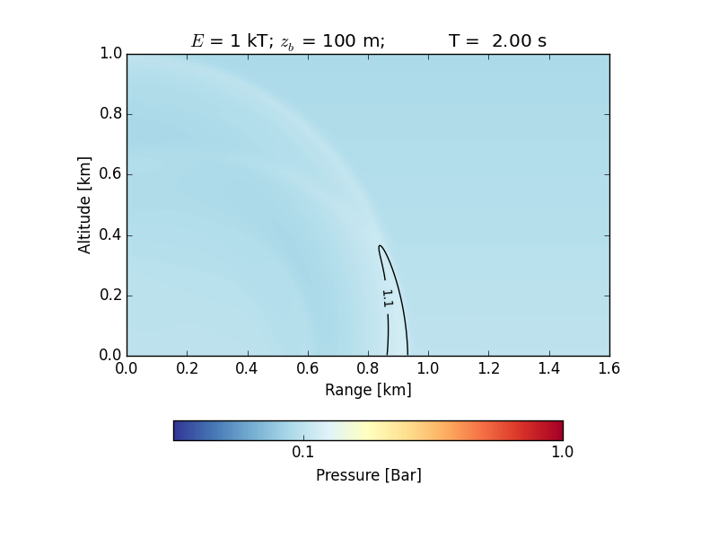
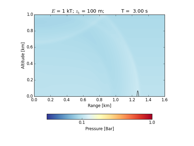
The images, which should be identical to those shown below, will be output to the directory @Plots/@. In addition, you will find the pdf document “MaxOverpressureVsRange” that includes a plot of the maximum overpressure as a function of range from the model in comparison with experimental data described by Glasstone and Dolan (1964).

The atmosphere is treated like any other layer in the model, so the pressure (and density) gradient in the air is computed from the top down. For this reason, @P_SURF@ in this case defines the pressure at the top of the model, not the surface.

--------- Set pressure at the top of the mesh appropriate
--------- to achieve 1 bar at the bottom
P_SURF      Pressure at top of mesh       : 0.9D5

As we are using a very low-density material, we must turn off the density cutoff:

--------- Make sure density cut-off is zero to retain all matter
ROCUTOFF    density Cut off               : 0.0

The airburst is initiated by depositing internal energy in the object. To do this we need to define the specific internal energy in the object, which is distributed uniformly. This is calculated by dividing the desired airburst energy (1 kTon) by the mass of the air in the object.

--------- This is the sp. int. energy required for a 1 kT explosion
OBJENER     specific internal energy      : 2.1085023D7

By default, objects are placed above the top 'layer'. To move the airburst object to the appropriate altitude we offset it downwards.

--------- Shift the bottom of the sphere down from top of mesh (layer)
--------- so that the centre is at 100-m altitude 
---------                         = ( 1 + 100m/dx - OBJRESH - LAYPOS)
OBJOFF_V    proj offset (ver)             : -234

If any boundary is open the atmosphere will slowly flow out of it. Instead we use a no normal flow (free-slip) boundary condition on all sides.

BND_L       left                          : FREESLIP
BND_R       right                         : FREESLIP
BND_B       bottom                        : FREESLIP
BND_T       top                           : FREESLIP

Here we use an array of Eulerian probes (fixed in space; PARRAY_T = EULER) to record the pressure in the air as a function of range. We use a single probe array PARRAY_N = 1, vertically located in the bottom row of cells in the mesh PARRAY_V = 1. The first probe in the array is in the first column of cells (PARRAY_O = 0) and the probes are spaced two cells apart (PARRAY_S = 2) until the last probe in the 400th column (PARRAY_B = 400).

PARRAY_N    number of arrays              : 1
PARRAY_V    first array                   : 1
PARRAY_T    fixed/Moving in space         : EULER
PARRAY_O    first probe                   : 0
PARRAY_S    probe spacing                 : 2
PARRAY_B    last probe                    : 400

As we treat the air as an inviscid fluid we can deactivate the deviatoric stress model.

STRESS      Consider stress               : 0

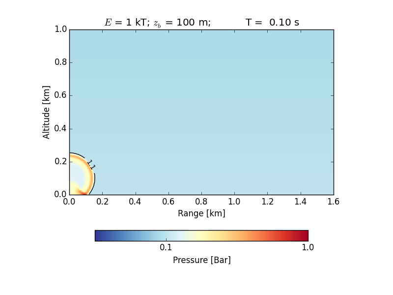
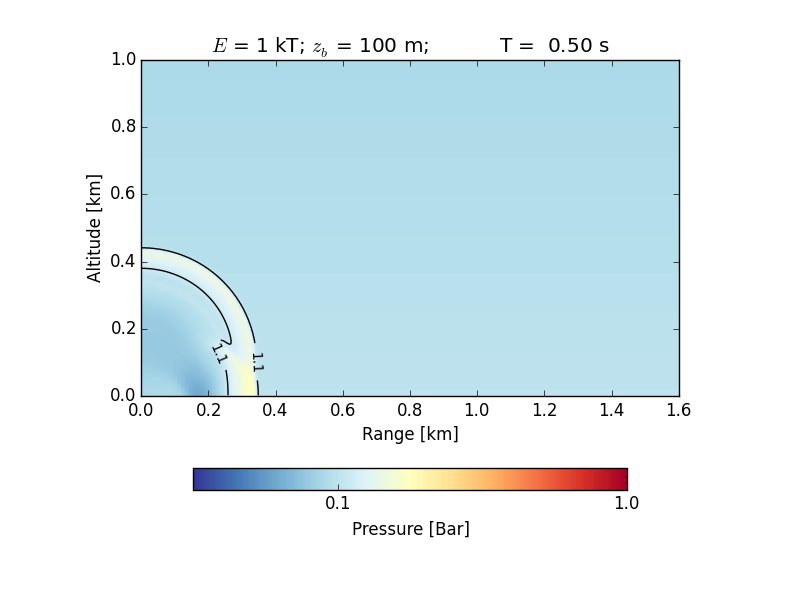
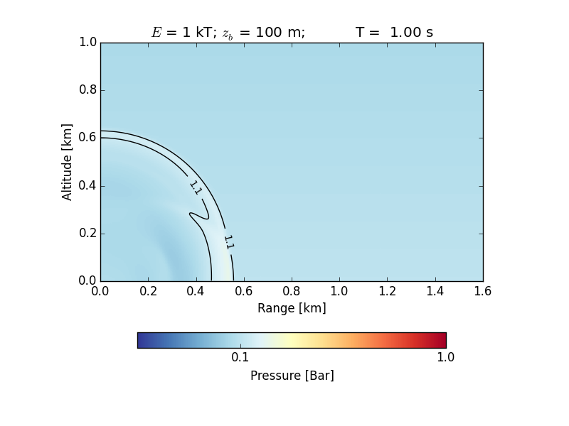
The figures below show (1) a time series of the propagation of the shock wave in air and its decay (in black you see the envelope of the region with 1.1 bar or higher; note the reflections from the ground at ~0.1 s); and (2) the maximum overpressure versus the range in comparison with experimental data.