Nick Goldman explains the Goldman-Cox (GC) test in this paper

The basic idea is that we are asking whether the full model (i.e. the tree, branch lengths, model parameters, everything we estimate from the data) is an adequate description of the data. We do this by calcualting the cost of the model, which is just: the maximum liklelihood of the data under the model, minus the unconstrained likelihood (see below). We'll call this delta. You can read Nick's paper for a full description of this, but he puts it rather nicely on page 184:

[delta] can be considered the "cost" of using [our model assumptions] to make 
inferences about phylogeny. A low cost indicates that [our model] is adequate; 
a high cost indicates that [our model] is performing badly and should be rejected.

Be warned! For most datasets, you will reject the full model. This is simply because most modern datasets are large, and most of our models of evolution are still really simple. So we should expect to reject them. This doesn't mean they don't produce useful inferences, of course!

Calculating the cost of the model is easy, but to interpret it we need to know if the cost is surprisingly large or small. That is, we need some idea of the null distribution of costs. One way to do this, and the method used by the Goldman-Cox test, is to use a parametric bootstrap. A parametric bootstrap is a really useful way to ask questions in phylogenetics. The absolute classic paper on this is from Goldman, Anderson, and Rodrigo in 2000. You should read this first. There are many flavours of parametric bootsrap in phylogenetics, but they all follow the same pattern:

1. Do an analysis on your focal dataset (probably your empirical dataset), and measure the thing you're interested in (here it's delta)
2. Call the model you estimated from your empirical dataset the null model, then simulate a lot of new datasets using that null model
3. Measure the thing you are interested in on each of the simulated datasets (here it's delta)
4. Ask if your observed value (from step 1) is surprising given the list of simulated values (from step 3)

In other words, for the Goldman-Cox test we can figure out if our observed cost is high, by simulating lots of cost values under the null model, and then re-calculating the cost on those. That null distribution tells us what kind of cost values we should expect when the null model is true. And so it then allows us to ask whether our observed value looks plausible. If you're a biologist and you like working with an alpha value of 5%, you might consider that if your observed cost is in the highest 5% of the simualted costs, you should reject your model as inadequate.

The Goldman-Cox test doesn't (and can't) tell you which aspects of your model might be causing the most trouble. But it's a really good place to start when considering how well you are able to to model your data.

For this recipe I'll use data from the Bovidae family with five taxa (Yak, Cow, Goat, Sheep and Antelope) and 5,000 sites. This is a (very) small subset of the amazing Wu et al 2018 dataset. I keep the file to 5K sites because that helps keep the file sizes manageable and analyses fast for a demonstration.

Note: for this version of the Goldman-Cox test, you can only use alignments with no gaps or ambiguities. So I have removed any sites with gaps or ambituities from the alignment.

• bovidae_4K.phy, our input alignment of 5 taxa and 5,000 sites.

All of the work in IQ-TREE can be done in a single commandline, thanks to the magic of AliSim.

Here's the commandline, and below I deconstruct the options:

iqtree -s bovidae_4K.phy --alisim simulated_MSA --num-alignments 999

• -s bovidae_4K.phy: tells IQ-TREE to do a standard analysis on the bovidae_4K.phy file, where it chooses the model, estimates the tree and model parameters
• --alisim simulated_MSA tells AliSim to then simulate alignments that mimic this alignment (i.e. use the tree and model parameters estimated from the original data)
• --num-alignments 999 tells AliSim that we want 999 mimicked alignments (999 is a good number for a parametric bootstrap)

The bovidae_4K.phy.iqtree file, gives us the information we need to calculate delta:

Log-likelihood of the tree: -6545.5196 (s.e. 74.4412)
Unconstrained log-likelihood (without tree): -6448.4561

So delta here is: -6448.4561 - -6545.5196 = 97.0635

Let's write a little bash function to calculate this value - it will help us in the next step we have to do the same for the 999 simulated datasets. The first couple of lines of this function just get the two likelihood values we want. Then we take the difference to get delta. Of course, you can do this in whatever language you like. But I like bash, so here's my attempt:

get_delta () {
    # a function to get the difference bewteen lnL and unconstrained lnL from a .iqtree file
    # assumes that the only passed argument is the name of a .iqtree file

    lnL_model=$(grep "Log-likelihood of the tree: " $1 | awk '{print $5}')
    lnL_unconstrained=$(grep "Unconstrained log-likelihood" $1 | awk '{print $5}')
    delta=$(echo $lnL_unconstrained - $lnL_model | bc) 

    echo $delta
}

Now if you copy-paste that function into your bash terminal, then run

get_delta bovidae_4K.phy.iqtree 

You should get the output 97.0635 or something quite close (it can vary depending on the random number seed)

Now we need get the 999 delta values from our simulated alignments. This will give us a null distribution for delta when the model estimated from the original dataset is true. In other words, this will tell us what kind of values of delta we should expect to see when our model really does have a single tree with the branch lengths we estimated, all the substitution model parameters we estimated, etc.

To get our delta values from our 999 simulated alignments, we'll first run IQ-TREE on each alignment in turn. We can do that in bash with a simple for loop. You can do this in whatever language you like, and in some situations you would want to parallelise this to make it faster. But for this tutorial I'll keep it as simple as possible (the below might take a few minutes to run):

for alignment in simulated_MSA_*.phy; do
     iqtree -s $alignment
done

The first line in that loop just uses the wildcard * to match all of the simulated alignment files in turn. Then the second line runs IQ-TREE on each alignment.

Now we've done the analysis, we need to get all of our delta values from those output files. We can do this using the get_delta() function we wrote above, in a for loop just like the one we used to run IQ-TREE. The for loop below just uses >> to put all the delta values into a file called simulated_delta.txt:

for iqtree_file in simulated_MSA_*.phy.iqtree; do
     get_delta $iqtree_file >> simulated_delta.txt
done

If you look through your list of deltas in the simulated_delta.txt file, you'll see they all seem to be below the observed value. So, if we were to order the list of the 999 simulated deltas and our observed delta from largest to smallest, our observed delta would be in position 1 out of 1000 in the list. So we know our p-value here would be at most 1/1000, i.e. p<=0.001. In other words, we can reject the hypothesis that the full model (tree, branch lengths, substitution model etc) is an adequate description of the data...

Not all analyses will be quite this obvious, so here's a little R script that you could use to calculate the p-value:

library(ggplot2)
# reads the simulated deltas into a data frame
simulated_deltas = read.delim("simulated_delta.txt", header=F)

# the p-value is just the position of the observed value in the ranked list,
# divided by the list length

# first we tell R our observed value of delta from above
observed = 97.0635

# the position is just the length of the list if you'd added the observed value (1000 in our case)
# minus how many of the simulated values are smaller than the observed value
position = (nrow(simulated_deltas) + 1) - sum(observed>simulated_deltas$V1)

# the p-value is just the position divided by teh length of the list if you'd added the observed value
p_value = position / (nrow(simulated_deltas) + 1)

p_value

# then we can make a plot to help us visualise it
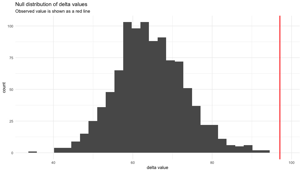
ggplot(simulated_deltas, aes(x=V1)) + 
    geom_histogram() + 
    geom_vline(xintercept = observed, colour="red", size=1) +
    theme_minimal() +
    xlab("delta value") +
    ggtitle("Null distribution of delta values", subtitle = "Observed value is shown as a red line")

In this case, you'd get the answer 0.001. Since we're at the very extreme of the distribution here, we can go one better than saying that the p-value equals 0.001, and say that it is at most 0.001, i.e. p<=0.001.

And our histogram helps make this clear.

Last tested with IQ-TREE 2.2.0.3