Interpolation - incanter/incanter GitHub Wiki

Problem: given a set of points:

Need to construct a function that contains given points.

There are infinite number of solutions. 2 example solutions that satisfy our conditions:

This is what interpolation all about. Interplotaion is a construction of a function that contains predefined set of points in 2d and 3d (actually any D but we work only with 2 and 3). This is not a strict math definition. For strict definition check Wikipedia article. There are infinite number of ways to build interpolation functions. incanter-interpolation module provides following kinds of interpolation: linear spline, polynomial, cubic spline, cubic hermite spline, B-spline, linear least squares.

• API
• interpolate
  • Linear
  • Polynomial
  • Cubic
  • Cubic hermite
  • Linear least squares
• interpolate-parametric
  • Linear
  • Polynomial
  • Cubic
  • Cubic hermite
  • Linear least squares
  • B-spline
  • Common options
• interpolate-grid
  • Bilinear
  • Polynomial
  • Bicubic
  • Bicubic hermite
  • Linear least squares
  • B-surface
  • Common options

There are 3 public functions in incanter.interpolation namespace:

(interpolate points type & options)

(interpolate-parametric points type & options)

(interpolate-grid points type & options)

See next parts of the tutorial for detail description.

interpolate builds a function f(x) = y based on input points (x, y).

It supports following kinds of interpolation: :linear, :polynomial, :cubic, :cubic-hermite, :linear-least-squares.

Basic usage:

(require '[incanter.interpolation :refer :all])
            
(def ^:dynamic points [[0 0] [1 3] [2 0] [5 2] [6 1] [8 2] [11 1]])

(def interp (interpolate points :linear))

(interp 0)   ; 0.0
(interp 0.5) ; 1.5

Define function for plotting function as well as input points:

(require '[incanter
           [charts :as charts]
           [core :as core]])
           
(defn plot [fn]
  (-> (charts/function-plot fn 0 11)
      (charts/add-points (map first points)
                         (map second points))
      (core/view)))

Linear interpolation is the simplest kind of interpolation here. It's basically connects all points using straight lines. Wikipedia article.

(plot (interpolate points :linear))

Polynomial interpolation builds a polynomial of degree n-1 that contains all input points. Wikipedia article.

(plot (interpolate points :polynomial))

Polynomial interpolation is pretty unstable when n is not small. Let's use updated points vector with 3 new points:

(binding [points [[0 0] [1 3] [2 0] [3 3] [4 2] [5 2] [6 1] [7 4] [8 2] [11 1]]]
  (plot (interpolate points :polynomial)))

You can see that function has large negative values at the right side. Don't use polynomial interpolation for large n or choose xs for your points very carefully (you can use Chebyshev nodes).

Cubic spline is a piece-wise function that consists of cubic polynomials. Every pair of neighbours polynomials has same values on common border as well as first and second derivatives.

(plot (interpolate points :cubic))

Cubic spline can be little customised by specifying boundaries conditions:
1 Natural conditions (default). Second derivatives on left and right ends of a function are equals to 0.

(interpolate points :cubic :boundaries :natural)
; which is equilavent to 
(interpolate points :cubic)

(plot (interpolate :cubic :boundaries :closed))

Cubic Hermite spline similar to cubic spline. The difference is that it constructs function using values and first derivatives in given nodes. By default first derivatives are approximated and don't need to be passed explicitly. Wikipedia article.

(plot (interpolate points :cubic-hermite))

You can specify first derivatives explicitly:

; left image
(plot (interpolate points :cubic-hermite 
                          :derivatives [1 1 1 1 1 1 1]))
            
; right image
(plot (interpolate points :cubic-hermite
                          :derivatives [-1 -1 -1 -1 -1 -1 -1]))

Linear least squares (LLS) is not exactly interpolation but rather approximation of a set of points. LLS builds a linear combination of base functions such that sum of distances from input points to result function is minimal possible. Wikipedia article.
Example: let's approximate our points using quadratic polynomial.

; define basis functions
; basis functions defined as a function that takes 1 argument x and returns n values
; we want to get quadratic polynomial - it means we need basis functions 1, x, x^2
(defn basis [x] [1 x (* x x)])

(plot (interpolate :linear-least-squares :basis basis))

There are 2 built-in basis: polynomial and B-spline. Polynomial basis is 1, x, x^2, x^3, etc. About B-spline you can read in interpolate-parametric section. Example of usage:

; approximate points using linear equation
; to do this we need 2 basis functions: 1 and x
; so use built-in polynomial basis with 2 first functions:
(plot (interpolate :linear-least-squares
                   :basis :polynomial :n 2))

interpolate-parametric builds a parametric function f(t). This function defines a curve that contains input points. Function defined in range [0, 1].

It supports following kinds of interpolation: :linear, :polynomial, :cubic, :cubic-hermite, :linear-least-squares, :b-spline.

(require '[incanter.interpolation :refer :all])

(def points [[0 10] [2 13] [4 10] [2 5] [0 0] [-2 5] [-4 10] [-2 13] [0 10]])

(def interp (interpolate-parametric points :linear))

(interp   0) ; [0 10]
(interp 0.5) ; [0  0]
(interp   1) ; [0 10]

Define function for plotting parametric function as well as input points:

(require '[incanter
           [charts :as charts]
           [core :as core]])
           
(defn plot [fn]
  (-> (charts/parametric-plot fn 0 1)
      (charts/add-points (map first points)
                         (map second points))
      (core/view)))

(plot (interpolate-parametric points :linear))

(plot (interpolate-parametric points :polynomial))

Chebyshev nodes are used in parametric interpolation so result function is pretty stable.

; natural boundaries conditions (left image)
(plot (interpolate-parametric points :cubic))

; closed boundareis conditions (right image)
(plot (interpolate-parametric points :cubic :boundaries :closed))

(plot (interpolate-parametric points :cubic-hermite))

You can also use :derivatives option as in interpolate.

(plot (interpolate-parametric points :linear-least-squares :basis :polynomial :n 2))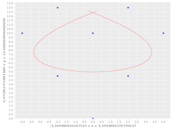 

B-spline is another kind of approximation. It constructs smooth curve resembling input points. Wikipedia article.

(plot (interpolate-parametric points :b-spline))

You can control "smoothness" by specifying spline degree:

(doseq [degree [1 2 3 (count points)]]
  (plot (interpolate-parametric points :b-spline :degree degree)))

Default degree is 3.
If degree is equals to number of points then B-spline becomes Bezier curve.

You can change parameter range from [0, 1] to whatever you want by using :range options:

(def interp (interpolate-parametric points :linear :range [-1 1]))

(interp -1) ; [0 10]
(interp  0) ; [0  0]
(interp  1) ; [0 10]

interpolate-grid is similar to interpolate-parametric but uses grid of points. It is defines function f(x,y) that defines surface. Default function range is [0, 1]x[0, 1].

It supports following kinds of interpolation: :bilinear, :polynomial, :bicubic, :bicubic-hermite, :linear-least-squares, :b-surface.

(require '[incanter.interpolation :refer :all])

(def grid [[0 1 2]
           [3 4 5]
           [6 7 8]])

(def interp (interpolate-grid grid :bilinear))

(interp    0   0) ; 0.0
(interp    1   1) ; 8.0
(interp  0.5 0.5) ; 4.0
(interp 0.25   1) ; 6.5

Incanter has no support for viewing surfaces so there will be no function. For viewing was used quil with HE_Mesh. Check this app.

Note that grid used in code examples and grid used in image examples are different.

(interpolate-grid grid :bilinear)

(interpolate-grid grid :polynomial)

(interpolate-grid grid :bicubic)

(interpolate-grid grid :bicubic-hermite)

You cannot specify custom derivatives as in interpolate function. It's not hard to implement I just not sure what API should look like because it's neccessary to specify following matrices of derivatives: dx, dy, dxdy. If you have an idea or need this option - create an issue.

Following basis is used: 1, x, y, sin(x), cos(x), sin(y), cos(y)

(interpolate-grid grid :linear-least-squares
                       :basis (fn [x y] [1 x y (Math/sin x) (Math/cos x) (Math/sin y) (Math/cos y)]))

There is 1 built-in basis: polynomial: 1, x, y, x^2, xy, y^2, x^3, etc:

(interpolate-grid grid :linear-least-squares
                       :basis :polynomial :n 5)

(interpolate-grid grid :b-surface)

:degree option is available.

By defaul surface is defined on range [0, 1]x[0, 1]. You can change it using :x-range, :y-range or :xs, :ys options.

:x-range, :y-range is similar to :range option in interpolate-parametric function. It allows to change range from [0, 1]x[0, 1] to whatever you want.

(def grid [[0 1 2]
           [3 4 5]
           [6 7 8]])

(def interp (interpolate-grid grid :bilinear :x-range [0 10] :y-range [0 10]))

(interp  0  0) ; 0
(interp 10 10) ; 8 

:xs, :ys allows to specify points explicitly.

If grid has size 3x3 you have to specify 3 values for xs and 3 values for ys:

(def interp (interpolate-grid grid :bilinear :xs [0 1 2] :ys [10 20 30]))

(interp 0 10) ; 0
(interp 2 30) ; 8