GVRS Jump Start 01_Reading GVRS files - gwlucastrig/gridfour GitHub Wiki
Introduction
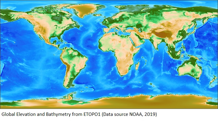
We begin this series of articles on GVRS techniques by describing how to read data from a GVRS file. For the examples that follow, we will use a GVRS file created from the ETOPO1 data set. ETOPO1 is a whole-Earth elevation and ocean-depth product that was created by the U.S. government's National Oceanographic and Atmospheric Administration (NOAA). It is available in the public domain and can be used free of charge. For this article, we used the open-source GVRS API to make a faithful transcription of the data from ETOPO1. If you would like to obtain the GVRS-formatted version of ETOPO1, you may download it from ETOPO1_v1.0.4.gvrs
Here are a few statistics about the ETOPO1 data source:
- Grid size 10800 rows by 21600 columns
- 233 million data cells
- Geographic (latitude, longitude) coordinates
- Cell spacing 1 minute of arc (1/60th of a degree)
- Elevation and depth given in meters
- Download size for GVRS compressed version: 125 MB.
The picture below was derived using the GVRS API to process the elevation and bathymetry information in the ETOPO1 data set. To produce the image, the source data was down sampled by a factor of 30-to-1.
Opening a file
The code snippet below illustrates the steps in opening a GVRS file.
File file = new File("ETOPO1_v1.0.4.gvrs");
try (GvrsFile gvrs = new GvrsFile(file, "r")) {
  gvrs.summarize(System.out, false);
} catch (IOException ioex) {
  System.out.println("IOException for " + file.getName() + ": " + ioex.getMessage());
}
The GvrsFile class is the main class for accessing GVRS files. An application opens a GVRS file in much the same way it would open a conventional file using one of the Java standard API's file-related classes such as a FileInputStream. The GvrsFile class implements Java's Closeable interface, so it can be enclosed in a Java try-with-resource block. Enclosing file-access code in a try-with-resources block ensures that the file will be properly closed and its resources freed up when the code exits the block. It is the preferred way to handle files both in Java's standard API and in the GVRS API.
The code snippet doesn't do much except to print a summary of the file organization to standard output. The text below gives an edited view of the summary for ETOPO1_v1.0.4.gvrs
GVRS Raster File:   ETOPO1_v1.0.4.gvrs
UUID:               0eb855f0-aa4c-4c5f-a660-1fb8b4201a50
Identification:     ETOPO1_Ice_c_gmt4.grd

Rows in Raster:           10800
Columns in Raster:        21600
Cells in Raster:      233280000

Range x values:      -179.991667,  179.991667, (359.983333)
Range y values:       -89.991667,   89.991667, (179.983333)
Data compression:       enabled

Elements
   Name   Type    Description
   z      SHORT   Elevation (positive values) or depth (negative), in meters
Identification data
The first thing we see in the summary text are identification strings.
All GVRS files are automatically assigned a Universally Unique Identifier (UUID). For practical purposes, the UUID assigns a unique identifier to every GVRS file. This feature is intended to support tracking files in inventory control systems, databases, and similar applications.
Every GVRS file can carry an optional, arbitrary identification string. The Gridfour software distribution includes a demonstration application called PackageData.java which uses the root-name of the source-file as its identification.
The identification strings are followed by the dimensions of the grid. These value match the statistics I cited above.
GVRS elements
The most interesting item in the summary block may be the table of elements .
GVRS elements provide the primary access point for reading data from a GVRS file. A GVRS file can contain one or more elements. ETOPO1 contains only a single value per grid cell, so its GVRS file specifies just one element. When I built ETOPO1_v1.0.4.gvrs, I assigned this element the name "z". Names serve as a kind of key-string for referring to elements in a GVRS file.
The following code snippet shows an example of how we might read the value stored at grid row 1500 and grid column 1000. When GVRS methods accept grid coordinates, they are always given in the order row first and column second. In the example that follow, the GvrsElement object we obtained for the name "z" is used to access the underlying data and obtain a value at the specified coordinates.
File file = new File("ETOPO1_v1.0.4.gvrs");
try (GvrsFile gvrs = new GvrsFile(file, "r")) {
    GvrsElement zElement = gvrs.getElement("z");
    float value = zElement.readValue(1500, 1000);
}
When an application constructs a GvrsFile object, the GVRS API constructs a single GvrsElement instance for each element. Since ETOPO1 contains only one data value (elevation), the GvrsFile instance constructed from ETOPO1_v1.0.4.gvrs contains only a single GvrsElement instance. When required, however, the GVRS API supports multiple elements per file.
One thing that might be useful to note here is the way the GVRS API names its methods. Methods named get and set access objects that exist within the GvrsFile, but they do not change its data. Methods named read and write access or modify the content of the GVRS raster and may potentially trigger read or write operations for the associated data file.
Reading data
So far, the example code snippets haven't done anything particularly interesting. So let's look at an example that actually used the GVRS ETOPO1 file to retrieve elevation data for inhabited locations on the face of the Earth.
Look-up operations using geographic coordinates
For the example below, I created a simple class named Place that stores a name and a set of geographic coordinates (latitude and longitude). To create some sample data, I populated a set of Place objects with some arbitrarily chosen locations:
static Place[] places = {
    new Place("Auckland, NZ",                 -36.84,     174.74),
    new Place("Coachella, California, US",     33.6811,  -116.1744),
    new Place("Danbury, Connecticut, US",      41.386,    -73.482),
    new Place("Dayton, Ohio, US",              39.784,    -84.110),
    new Place("Deming, New Mexico, US",        32.268,   -107.757),
    new Place("Denver, Colorado, US",          39.7392,  -104.985),
    new Place("La Ciudad de México, MX",       19.4450,   -99.1335),
    new Place("La Paz, Bolivia",              -16.4945,   -68.1389),
    new Place("Mauna Kea, US",                 19.82093, -155.46814),
    new Place("McMurdo Station., Antarctica", -77.85033,  166.69187),
    new Place("Nantes, France",                47.218,     -1.5528),
    new Place("Pontypridd, Wales",             51.59406,   -3.32126),
    new Place("Québec, QC, Canada",            46.81224,  -71.20520),
    new Place("Sioux Falls, South Dakota, US", 43.56753,  -96.7245),
    new Place("Suzhou, CN",                    31.3347,   120.629),
    new Place("Zürich, CH",                    47.38,       8.543)
};
GVRS is not a Geographic Information System (GIS), but GVRS is useful for processing geophysical data sources. The GVRS API implements support for geographic coordinates as a convenience for developers working with geospatial information.
In the code snippet below, the geographic coordinates for the places are converted to integer grid coordinates and used to query elevations. Note that GVRS always gives geographic coordinates in the order latitude followed by longitude.
try (GvrsFile gvrs = new GvrsFile(file, "r")) {
    GvrsElement zElement = gvrs.getElement("z");
    GridPoint grid;
    for (Place place : places) {
        grid       = gvrs.mapGeographicToGridPoint(place.latitude, place.longitude);
        int row    = grid.getRowInt();
        int column = grid.getColumnInt();
        float z    = zElement.readValue(row, column);
        System.out.format("%-30s %7.2f,  %7.2f, %12.1f%n",
          place.name, place.latitude, place.longitude, z);
    }
}
The results are shown below (and, yes, the the town of Coachella California really is below sea level).
Name                              Lat         Lon       Elevation (m)
Auckland, NZ                    -36.840,    174.740,         15.0
Coachella, California, US        33.681,   -116.174,        -22.0
Danbury, Connecticut, US         41.386,    -73.482,        154.0
Dayton, Ohio, US                 39.784,    -84.110,        238.0
Deming, New Mexico, US           32.268,   -107.757,       1324.0
Denver, Colorado, US             39.739,   -104.985,       1602.0
La Ciudad de México, MX          19.445,    -99.134,       2240.0
La Paz, Bolivia                 -16.495,    -68.139,       3749.0
Mauna Kea, US                    19.821,   -155.468,       4044.0
McMurdo Station, Antarctica     -77.850,    166.692,         31.0
Nantes, France                   47.218,     -1.553,         22.0
Pontypridd, Wales                51.594,     -3.321,        129.0
Québec, QC, Canada               46.812,    -71.205,         28.0
Sioux Falls, South Dakota, US    43.568,    -96.725,        428.0
Suzhou, CN                       31.335,    120.629,          5.0
Zürich, CH                       47.380,      8.543,        435.0
Look-up operations using interpolation
The elevations shown in the table represent the value at the center of the grid cell that contains the specified coordinates. Since the spacing of the grid is approximately 1.85 kilometers (1.15 miles), the distance between the specified location and the elevation "point" could be more than a kilometer. To adjust for changes in elevation over distance, we use an interpolation method.
There are lots of ways to perform an interpolation. Each has their particular merits. For the GVRS project, we implemented an interpolation based on the B-Spline method. The code below shows an example. One thing to note is that the interpolator accepts GVRS "model coordinates" rather than latitudes and longitudes. Model coordinates are essentially Cartesian coordinates. So the interpolator accepts a value for longitude (e.g. the x coordinate) first and latitude (e.g. the y coordinate) second.
GvrsElement zElement = gvrs.getElement("z");
GvrsInterpolatorBSpline interpolator = new GvrsInterpolatorBSpline(zElement);
GridPoint grid;
for (Place place : places) {
    double zInterp = interpolator.z(place.longitude, place.latitude);
    grid           = gvrs.mapGeographicToGridPoint(place.latitude, place.longitude);
    System.out.format("%-30s %9.2f,  %9.2f, %12.1f%n",
      place.name, grid.getRow(), grid.getColumn(), zInterp);
}
The table below shows the results. Rather than showing latitude and longitude for the place names, it presents the computed grid coordinates. As we might expect, none of them are exact matches for row and column values.
Name                              Row      Column      Elevation (m)
Auckland, NZ                     3189.10,   21283.90,         15.2
Coachella, California, US        7420.37,    3829.04,        -20.9
Danbury, Connecticut, US         7882.66,    6390.58,        162.0
Dayton, Ohio, US                 7786.54,    5752.90,        242.5
Deming, New Mexico, US           7335.56,    4334.08,       1322.1
Denver, Colorado, US             7783.85,    4500.40,       1607.2
La Ciudad de México, MX          6566.20,    4851.49,       2238.9
La Paz, Bolivia                  4409.83,    6711.17,       3762.1
Mauna Kea, US                    6588.76,    1471.41,       3946.8
McMurdo Station, Antarctica       728.48,   20801.01,         83.5
Nantes, France                   8232.58,   10706.33,         15.4
Pontypridd, Wales                8495.14,   10600.22,        142.3
Québec, QC, Canada               8208.23,    6527.19,         23.9
Sioux Falls, South Dakota, US    8013.55,    4996.03,        428.3
Suzhou, CN                       7279.58,   18037.24,          6.1
Zürich, CH                       8242.30,   11312.08,        459.1
The value of interpolation
While the use of an interpolator adds an extra layer of interpretation to the data, it often represents a better way of modeling a surface. The difference between the two approaches – simple look up, and interpolation – can be summarized as follows:
- A simple lookup obtains the data value nearest to the query point.
- An interpolation provides an estimate of the actual value at the point of interest.
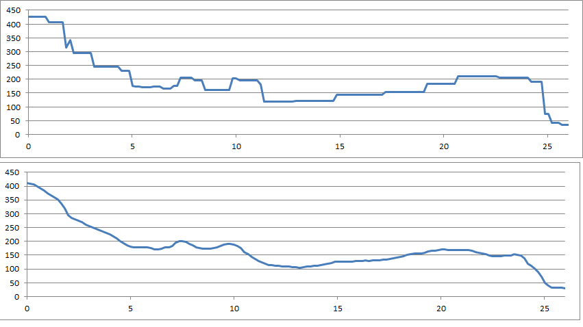
To get a sense of how surface modeling is affected by interpolation, consider the figure below. The figure shows the elevation profile for the route of the Boston Marathon with elevations in feet and distance traveled in miles. The Boston Marathon follows a set of paved roads starting in Hopkinton, MA and ending on Boylston Street in Boston, MA. The first frame shows the result using a simple lookup (nearest neighbor) without interpolation. The second frame shows the result using interpolation. Clearly, the interpolated profile is a closer match to how we would expect a road surface to behave.
Conclusion
This article introduced techniques used to access the data in a GVRS file. It is the first in a planned series of articles. In future articles I will provide more information about the GVRS API and offer suggestions on how to get the best results when using it.
As always, user feedback is a key to improving both the content of these wiki pages and the GVRS API itself. Got something to say? I'd be interested in hearing from you.
References
National Oceanographic and Atmospheric Administration [NOAA], 2019. ETOPO1 Global Relief Model. Accessed December 2019 from https://www.ngdc.noaa.gov/mgg/global/
University Corporation for Atmospheric Research [UCAR], 2019. NetCDF-Java Library Accessed December 2019 from https://www.unidata.ucar.edu/software/netcdf-java/current/