Note: This article makes frequent references to the Delaunay Triangulation and the Constrained Delaunay Triangulation. Readers who would like to get more background on these topics, may do so by searching the web or by looking at the two introductory articles at the wiki pages: About Delaunay Triangulations and What is the Constrained Delaunay Triangulation and why would you care?

Sometimes when building a Delaunay Triangulation for a surface, it is useful to partition the data into distinct regions. For example, a terrestrial elevation surface could be divided into regions of distinct vegetation types such grassland and forest. Since information about the vegetation type would not be directly supported by the geometry of the triangulated mesh structure itself, a supplementary data representation would be required to give a complete picture of the surface. In Tinfour, this requirement is addressed by polygon-based constraints. Polygon-based constraints give applications the ability to embed metadata for bounded regions into the structure of the Delaunay Triangulation.

In this tutorial we will look at the Tinfour Application Programming Interface (API) and review some techniques for taking advantage of the region-constraints. But before we do, let's take a look at a couple of examples.

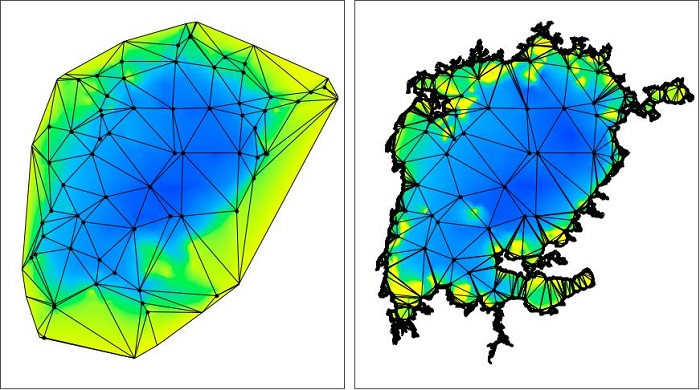
The picture below shows two examples of bottom-depth data for Africa's Lake Victoria. The panel on the left is a pure Delaunay Triangulation. The panel on the right is a Constrained Delaunay Triangulation in which the bottom depth sample points were supplemented with a polygon constraint based on the shoreline of the lake. The constraint allows the triangulation to include information about the true domain of the lake data. This technique was discussed at length in an earlier Wiki article. If you'd like to learn more about it, see Using the Delaunay to Compute Lake Volume.

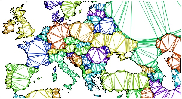
Here's another example of geographic data. In this case, the triangulation is entirely derived from region constraints derived from the Natural Earth Data geopolitical map data.

While all the examples so far have used geographic data sources, the Delaunay has much broader applications than its use in Geographic Information Systems (GIS). Here's a completely different kind of example:

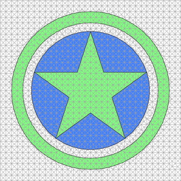
The Star graphic shown above will be the subject of our tutorial. You can find the code for it in the standard Tinfour source code distribution (see the file ConstraintStarDemo.java in the "demo" module). Here are the first few lines of code from the application:

// Define two lists, one to receive vertices, one to receive constraints
List<Vertex>      vertices    = new ArrayList<>();
List<IConstraint> constraints = new ArrayList<>();

// populate the elements to be added to the TIN
//    1)   a grid of vertices
//    2)   the constraint polygon in the form of a five-pointed star
//    3)   the 5 wedge-shaped polygons bordering the star
//    4)   a circular constraint enclosing the figure
//  
addGrid(vertices);
addConstraintStar(constraints);
addConstraintWedges(constraints);
addEnclosingRing(constraints);

// initialize the TIN, populating it with the elements to be presented
tin = new IncrementalTin(1.0);
tin.add(vertices, null);
tin.addConstraints(constraints, true);

The image shows an example of a Delaunay Triangulation based on a grid of vertices into which some geometric forms (a star, a ring) have been embedded. The addGrid() method in the example code populates a list of vertices with the points for that grid. The other "add" methods add polygon-based constraints (regions) to a list of constraints. We'll look at these methods below. For now, observe that the lists of vertices and constraints are used as the vehicle for adding vertices and constraints to the Constrained Delaunay Triangulation constructed using the IncrementalTin class (the class named includes the acronymn TIN, which stands for "Triangulated Irregular Network").

One thing to note here is that the IncrementalTin class requires that vertices be added before constraints. In fact, once constraints are added to the IncrementalTin, it can no longer accept additional elements. This behavior is due to limitations in the current Tinfour implementation and will be addressed in the future. For now, it is how the API has to be used.

Let's take a look at the first of the constraint-adding methods, addConstraintStar(). For a five-pointed star, the points are spaced at 72 degree intervals (360/5=72). The angle at each point is 36 degrees. The first point occurs at 18 degrees from the X-Axis. With that in mind, here's the code:

// Define angles and dimensions for building the constraints.
// The notches in the star have a radius of 1 unit.  The points have
// a computed radius of approximately 2.62 units.
final static double A18 = Math.toRadians(18);
final static double A36 = Math.toRadians(36);
final static double A72 = Math.toRadians(72);

final static double rNotch = 1.0;  // the inner radius
final static double rPoint = rNotch * (cos(A36) + sin(A36) * tan(A72));  // point radius

private void addConstraintStar(List<IConstraint> constraints) {
	// the polygon is given in counterclockwise order.
	PolygonConstraint p = new PolygonConstraint();
	p.setApplicationData(new Color(128, 255, 128));  // pale green
	for (int i = 0; i < 5; i++) {
	  double a = A18 + i * A72;
	  double x = rPoint * Math.cos(a);
	  double y = rPoint * Math.sin(a);
	  Vertex v = new Vertex(x, y, 0, iVertex++);  // a point
	  p.add(v);
	  a = A36 + A18 + i * A72;
	  x = rNotch * Math.cos(a);
	  y = rNotch * Math.sin(a);
	  v = new Vertex(x, y, 0, iVertex++);  // a notch
	  p.add(v);
	}
	p.complete();
	constraints.add(p);
}

The code defines a number of static variables for angles given in radians based on their corresponding measure in degrees. These angles are used to compute the Cartesian coordinates of the vertices in the five-pointed star polygon. The vertices are given as alternating points and notches. The five-pointed star was selected as an example because it demonstrates that a constraint polygon can be non-convex, just as long as it is not self-intersecting. Thus, a five-pointed star is valid polygon. A figure eight is not.

The loop above produces each of the five points and five notches in sequence. When the PolygonConstraint instance is fully populated, a call to the complete method indicates that it is finished and instructs the class to performs some internal bookkeeping related to the constraints geometry. At that point it is ready to be added to the list of constraints.

Note also that a Java Color object was added to the constraint as "application data". In Tinfour, all constraint implementations support the use of optional application data. This data can be anything that the application developer wishes to use. It could be an instance of a complex class containing several metadata elements, or it could be something much simpler, such as the single color specification used in this example. For the ConstraintStarDemo class, the image-rendering code uses the application data elements to set the color for each triangle embedded in a region constraint. I'll have more to say about rendering later in this article.

In addition to the five-pointed star constraint, the demonstration application also produces 5 circular wedge polygons that fit neatly into each notch of the star. These constraints are created in the addConstraintWedges() method. Although I won't include it here, the code for creating the wedges is very similar to that which creates the star. There's a good reason for that similarity. Tinfour does not permit polygon constraints to overlap, but it does allow them to share common edges. However, the API requires the vertices that form those edges have identical coordinates. It is critical that application code honors this requirement. If it does not, it will not be successful in its creation of adjacent constrained regions. Thus, in the demonstration application, the arithmetic for creating the Cartesian coordinates for the vertices that define common edges is identical.

Referring to the illustration of the star figure above, note that there is a thin black line marking the edges of all the constraint polygons. In Tinfour, edges in the Delaunay Triangulation carry information about any constraints with which they are associated. They also know whether an edge is the border of a constraint region or if it is one of the interior edges. When drawing edges for the TIN, the demonstration application uses the edge-to-constraint information to determine color.

You may have noticed that in the addConstraintStar() method, the code for creating the five-pointed star produced vertices in a counterclockwise order. This ordering reflects a very important point about region constraints. Tinfour assumes that the region defined by a polygon-based constraint lies immediately the the left of the edges on its border. So, when we visualize the construction of a polygon taken in counterclockwise order, it becomes apparent that the area to the left of each edge lies in the interior of the polygon.

So what happens when a polygon is constructed in clockwise order? The region defined by the constraint lies to the left of each edge, but the interior of the polygon lies to the right. So the interior of the clockwise polygon does not belong to a constrained region. In effect, the constraint defines a "hole" in that region.

This fact was used by the rendering logic to create the pale green ring surrounding the star. The outer circle of the ring is given in counterclockwise order, so the triangles immediately inside it are color-filled according to the Java Color object supplied by its application data. But the inner circle is given in clockwise order. Thus it serves to limit the extent of the filled area.

The image rendering logic for the five-pointed star was designed to illustrate how the Tinfour API allows an application to extract information about the polygon-based regions embedded in a Constrained Delaunay Triangulation. As I mentioned above, edges in a Tinfour triangulation can carry information about constraints. In the example triangulation, not all the edges carry such information. There are 4464 edges that are associated with the polygon constraints (either on the borders or in their interiors). But 3586 edges that have no association. When Tinfour builds triangles from these edges, it can extract information about the edge-to-constraint relationships and know whether the triangles themselves should carry a reference to a constraint.

To render the color-filled triangles, we take advantage of Tinfour's versatile TriangleCollector implementation. A detailed discussion of this implementation is given in the Tinfour Wiki article Tutorial Using TriangleCollector Techniques. The TriangleCollector depends on an application to provide an implementation of a Java "Consumer" that accepts objects of Tinfour's SimpleTriangle class. This arrangement is actually much easier to explain with code than to describe in writing. So here's the code for the Java Consumer in the Constraint Star Demo application:

static class TriangleRenderer implements Consumer<SimpleTriangle> {

	final Graphics2D g2d;
	final AffineTransform af;

	TriangleRenderer(Graphics2D g2d, AffineTransform af) {
	  this.g2d = g2d;
	  this.af = af;
	}

	@Override
	public void accept(SimpleTriangle t) {
		IConstraint constraint = t.getContainingRegion();
		if (constraint != null && constraint.definesConstrainedRegion()) {
			Object obj = constraint.getApplicationData();
			// The application data will always be a color object.
			// But this code checks the type anyway.
			if (obj instanceof Color) {
				g2d.setColor((Color) obj);
				Path2D path = t.getPath2D(af);
				g2d.fill(path);
				g2d.draw(path);
			}
		}
	}
}

The constructor for the TriangleRenderer accepts a Java Graphics2D element and an AffineTransform. The transform is used to map the Cartesian coordinates for the triangles to the pixel coordinates for the output image.

In the main body of the image-rendering logic, the triangle renderer is constructed and passed to the TriangleCollector as shown below:

Graphics2D g2d;       // drawing surface, populated by the application.
AffineTransform af;   // maps Cartesian coordinates to pixels.
TriangleRenderer triangleRenderer = new TriangleRenderer(g2d, af);
TriangleCollector.visitSimpleTriangles(tin, triangleRenderer);

The visitSimpleTriangles method constructs a SimpleTriangle instance for each triangle defined by the Triangulated Irregular Network (TIN). These triangle objects are passed into the TriangleRenderer's accept() method, which extracts constraint information and renders the triangle in the appropriate color. Those triangles that do not have constraint regions are not drawn.

In the discussion above, I mentioned that the borders of the constraints are drawn in black. Here's the loop for drawing the black edges:

g2d.setColor(Color.black);
for (IQuadEdge e : tin.edges()) {
	if (e.isConstrainedRegionBorder()) {
		e.setLine2D(af, l2d);
		g2d.draw(l2d);
	}
}

The demonstration code presented in this tutorial does not get constraints directly from Tinfour edge objects. Tinfour's IIncrementalTin classes preserve edge-to-constraint relationships and provide and API for obtaining them. Note that the edge classes themselves do not implement methods for getting the constraint references. The references are obtained using the IIncrementalTin instance. The rationale for this design choice is based on the need for a memory-efficient representation of edges. Tinfour was designed to support applications that build TIN structures with millions of vertices. And such large TINs contain a correspondingly large number of edges. Because of that, the design of the edge classes themselves are very lean. They do not have room for references to constraint objects. Instead, the edge-to-constraint mappings are stored in the containing IIncrementalTin class. Thus the internal logic for extracting constraint references is somewhat indirect. It requires the participation of the IncrementalTin instance itself. Here are some example code snippets showing how it is done:

// To get the constrained region to the left of an edge
if (e.isConstrainedRegionBorder()) {
	IConstraint constraint = tin.getRegionConstraint(e);
}

// To get the constrained region to the right of an edge,
// you must use the edge's dual
IConstraint constraint = tin.getRegionConstraint(e.getDual());

// If the constraint is in the interior of a region, then 
// both sides of it will have the same constraint
if (e.isConstrainedRegionInterior()) {
	IConstraint constraint = tin.getRegionConstraint(e);
}

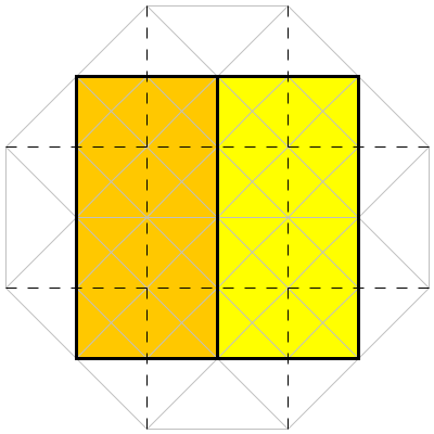
We'll leave off with one last example. In addition to region-based constraints, Tinfour also supports line-based constraints. Line-based constraints consist of a series of vertices that connect in an open line rather than a closed polygon. For terrestrial applications, they are often used to represent features such as roads, cliffs, or small rivers that are not well suited to representation by polygons. It is possible to mix both kinds of constraints together in a TIN. Where appropriate, line constraints can be contained inside polygon constraints. In fact, a line constraint is allowed to intersect a polygon constraint (or another line constraint), provided that the points of intersection are given as valid Vertex objects and included in both constraints.

The figure below shows an image that is output by the MixedModeConstraintTest.java class. The dashed lines represent linear constraints. The filled rectangles are, of course, region constraints supplied by the PolygonConstraint class. The linear constraints are allowed to cross in and out of the polygons because both the lines and polygons include matching vertices at the points of intersection. The styling for the drawing operations is based on application data that was stored as part of the constraints. MixedModeConstraintTest writes an output file called "test.png" to the local disk wherever it is run. It also performs a series of tests and inspections on the structure of the TIN that it produces. These tests exercise a lot of the Tinfour API elements and, as such, provide a good example of how they may be used.

One of the ideas that this tutorial was intended to convey is the versatility of region-based constraints. They can be used to support a wide variety of applications including both geographic and physical modeling as well as more abstract ideas. I hope that this tutorial, and the example code included in the Tinfour software distribution, will provide you with a good start for mastering these API elements.