PID - guidosassaroli/controlbasics GitHub Wiki
Proportional-Integral-Derivative (PID) control is the most widely used control algorithm in industrial applications, and its universal acceptance stems from two key factors: robust performance across a broad range of operating conditions and a straightforward implementation that simplifies its use by engineers.
As the name implies, the PID algorithm is built around three fundamental components—proportional, integral, and derivative terms. These parameters are adjusted to achieve an optimal system response.
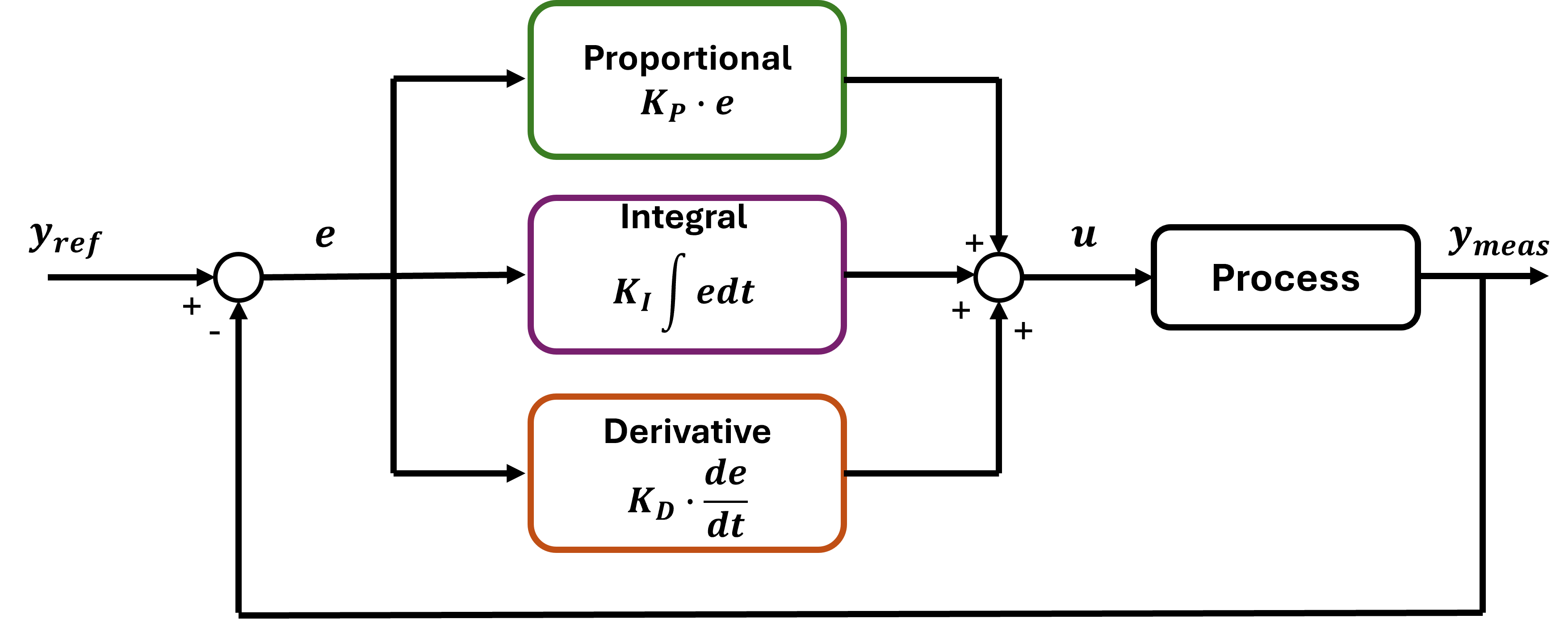
The basic form of a PID controller can be described with this differential equation:
$$ u = K_{P} \cdot e + K_{I} \int e , dt + K_{D} \frac{de}{dt} $$
Where $e$ describes the control error, i.e., the difference between the setpoint and the actual value of the controlled variable, and $u$ is the control action.
The individual components are described with independent parameters $K$.
A common alternative form is:
$$ u = K_{P} \left( e + \frac{1}{T_{I}} \int e , dt + T_{D} \frac{de}{dt} \right) $$
Where the proportional component is described unchanged by proportional gain $K_P$, but the integral component is defined by the integration time $T_I$ and the differential component by the derivative time $T_D$. Both newly introduced parameters have the dimension of time.
Proportional Response
The proportional component depends only on the difference between the setpoint and the process variable. The proportional gain ($K_P$) determines the ratio of output response to the error signal. For instance, if the error term has a magnitude of 10, a proportional gain of 5 would produce a proportional response of 50.
Integral Response
The integral component sums the error term over time. The result is that even a small error term will cause the integral component to increase slowly. The integral response will continually increase over time unless the error is zero, so the effect is to drive the steady-state error to zero.
Remark: A phenomenon called integral windup results when integral action saturates a controller without the controller driving the error signal toward zero. The next section introduces anti-windup PID.
Derivative Response
The derivative component causes the output to decrease if the process variable is increasing rapidly. The derivative response is proportional to the rate of change of the process variable.
PID Tuning
In general, increasing the proportional gain will increase the speed of the control system response. However, if the proportional gain is too large, the process variable will begin to oscillate. If $K_P$ is increased further, the oscillations will become larger and the system may become unstable or oscillate out of control.
A larger integral gain results in faster error correction but also larger overshoots and oscillations. A smaller integral gain results in a more stable response but also larger steady-state error and longer settling time.
Increasing the derivative time ($T_D$) parameter will cause the control system to react more strongly to changes in the error term and will increase the speed of the overall control system response. Most practical control systems use very small derivative times because the derivative response is highly sensitive to noise in the process variable signal. If the sensor feedback is noisy or if the control loop rate is too slow, the derivative response can destabilize the system.
Anti-Windup PID
In a standard PID controller, the integral part keeps accumulating error over time. This is great for eliminating steady-state errors, but it can also cause a problem known as integral windup.
Integral windup happens when the controller output is saturated but the integral term keeps accumulating error as if nothing is wrong. This causes overshoot, slow recovery, and unstable behavior. Basically, the controller is "trying too hard" and doesn’t realize it’s already doing all it can.
Anti-windup is a technique used to limit or correct the integral term when the controller output is saturated. It keeps the integral part from accumulating error that it can’t act on.
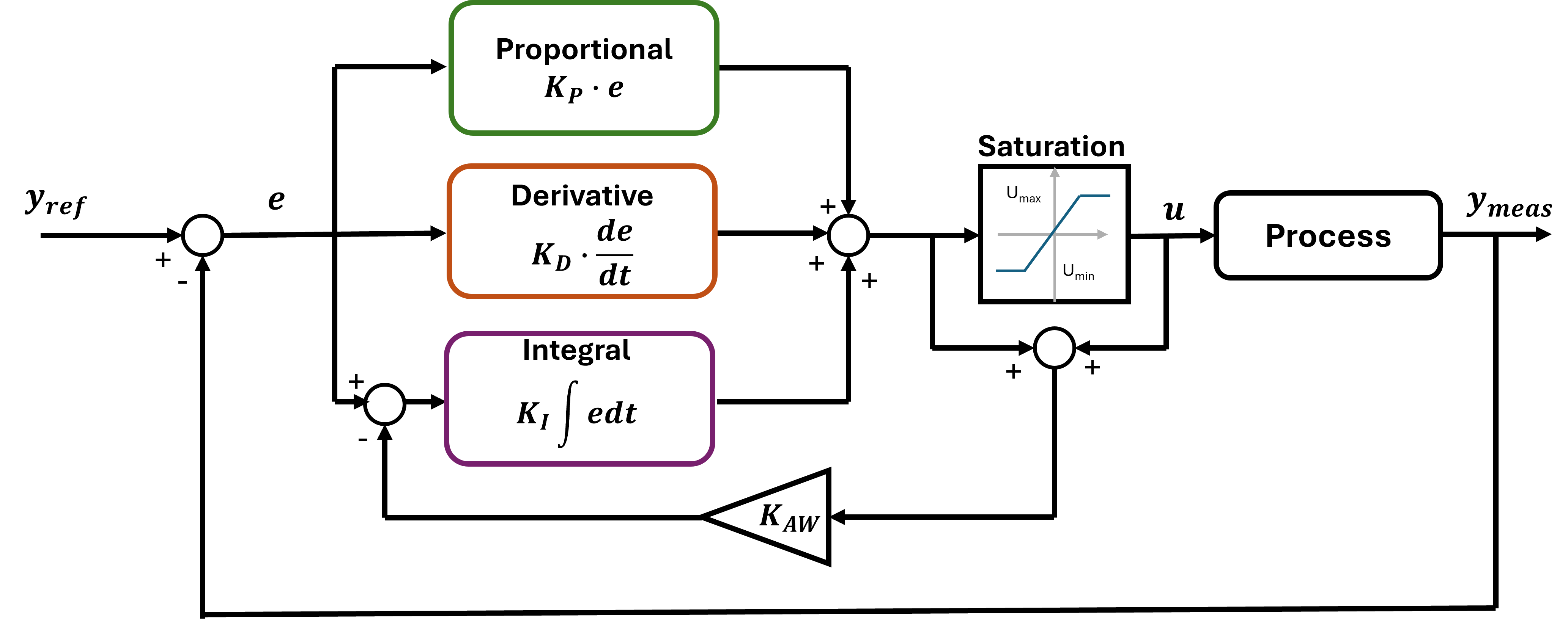
There are a few common methods, but a popular one is:
-
Clamping Method (Conditional Integration):
If the controller output is within limits, integrate normally.
If the output is saturated, pause or limit the integral update. -
Back-Calculation Method:
Adjust the integral term based on how far the controller output is from the desired (unsaturated) output.
Both methods aim to protect the controller from the adverse effects of windup, but they do so in different ways. Clamping works by halting integration under specific conditions, while back-calculation continuously adjusts the integrator in response to saturation. The choice between them often depends on the system dynamics, the frequency of saturation, and the desired smoothness of the control response.
Example
In the PID.ipynb file, you can find the design of a PID controller for temperature regulation in a room. The room is modeled by considering the contribution of heating from the heater and cooling due to the environmental temperature.
The temperature change is modeled as:
$$ \frac{dT}{dt} = k_{heat} \cdot P(t) - k_{cool} (T(t) - T_{env}) $$
Discretizing the differential equation, we obtain:
$$ T_{\text{next}} = T_{\text{current}} + (k_{heat} \cdot P - k_{cool}(T - T_{env})) \cdot \Delta t $$
This is a good simplification, as the focus of the example is the implementation of the controller.