MPC - guidosassaroli/controlbasics GitHub Wiki
Model Predictive Control (MPC) is a widely used control strategy in engineering and control theory, where it can be applied to a wide range of systems, including mechanical, electrical, and chemical processes. One key advantage of MPC is its ability to handle constraints on the system variables, such as limits on input and output variables, while still achieving optimal control performance. MPC also provides a framework for handling uncertainties in the system, through the use of robust optimization and adaptive control techniques.
Linear MPC
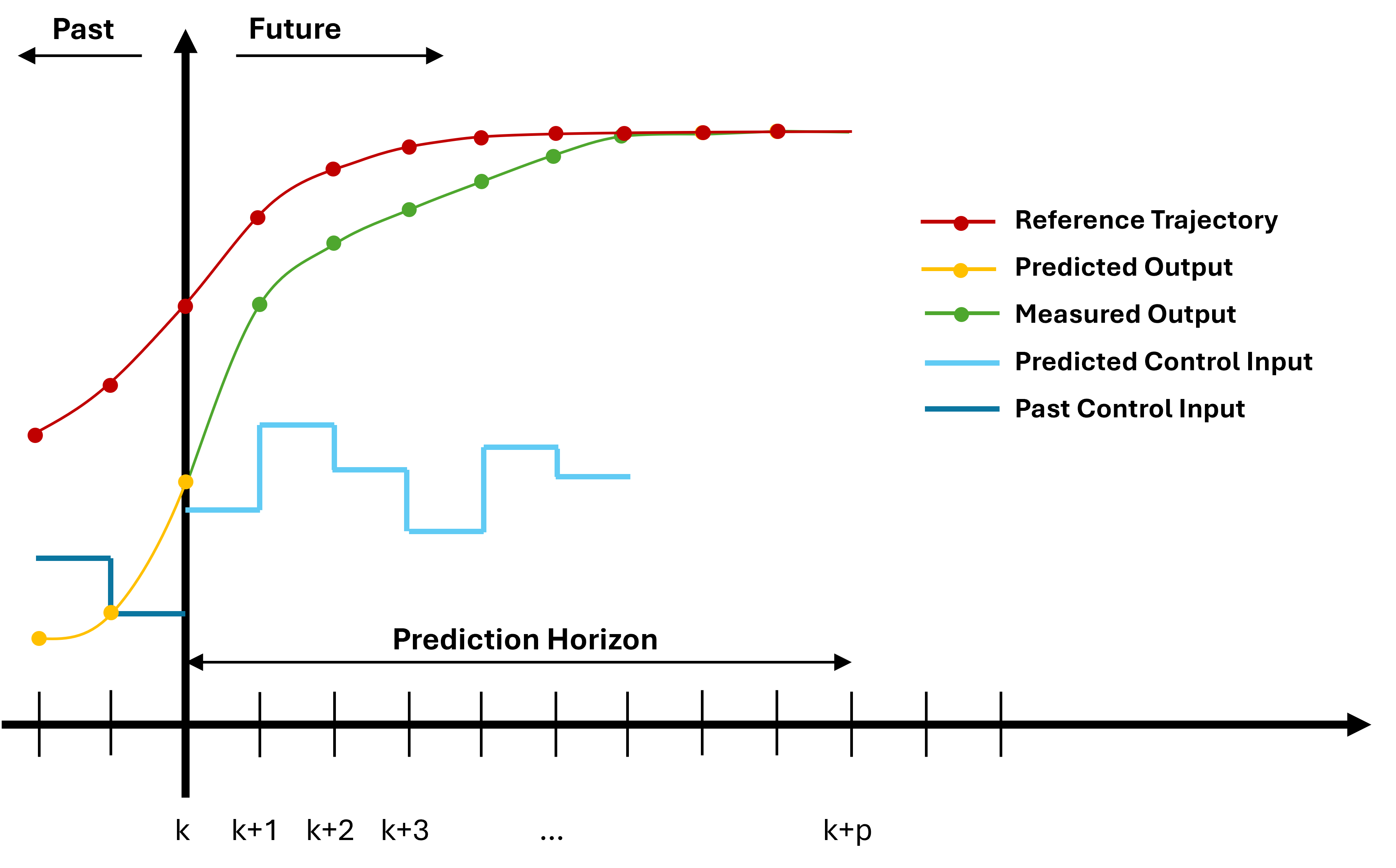
The objective of MPC is to find the best control sequence over a future horizon of N steps. In particular Linear MPC uses linear process models and optimizes linear or quadratic performance objectives with linear constraints. The following equation describes a quadratic cost function:
$$ l(x,u) = || x - x_{ref} ||_Q^2 + ||u||_R^2 $$
The equation represents the stage cost where
- $x$ - states at current time
- $x_{ref}$ - reference trajectory
- $u$ - inputs
- $Q$ - penalizing cost matrix for states
- $R$ - penalizing cost matrix for input
The cost function can be written as a combination of running cost as shown here:
$$ J_N(x(t),u(\cdot|t)) = \sum_{k=0}^{N-1} l(x(k|t),u(k|t)) $$
Hence, the MPC is characterized by the solution of the following optimization problem:
$$ V_N(x) = \min_{u} J_N(x,u) $$
Furthermore, the cost function must be minimized respecting the constraints on states and control actions: $$ x_{min} \leq y_k \leq x_{max} $$
$$
u_{min} \leq u_k \leq u_{max}
$$
The following Algorithm explains how the MPC works. It receives as input the objective function $J_N$, the dynamic prediction model $f(x,\dot{x}, u)$, the horizon $T$ and the initial guess $\hat{u}_{1:T}$, that is the previous solution of the MPC.
MPC Algorithm
1.  u₁:T ← 𝑢̂₁:T
2.  x_init ← GetCurrentState
3.  x_ref ← GetReferenceTrajectory
4.  u₁:T ← SolveOptimizationProblem(J_N, f, x_init, x_ref, T, 𝑢̂₁:T)
5.  u ← First(u₁:T)
6.  ApplyInput(u)
Hints: A good procedure is to use the control sequence of the previous step to warm-start the algorithm and speed it up, that's why in line 4 of Algorithm \ref{alg:MPC} $u_{1:T}$ is given as input to the SolveOptimizationProblem function. By providing a good initial guess for the control input, the solver can start the optimization process from a point that is already close to the optimal solution. This can lead to faster convergence and improved control performance. In each iteration, the previous control input trajectory is used as an initial guess for the current iteration, taking advantage of the continuity and smoothness of the control signal.
Nonlinear MPC
Nonlinear model predictive control (NMPC) is the nonlinear counterpart of MPC and it has been applied to a wide range of complex systems. NMPC combines the predictive power of model-based control with the ability to handle nonlinear systems, making it a popular choice for many applications. The book by Rawlings, Mayne and Diehl \cite{MPCbook} provides an excellent overview of NMPC, including its mathematical foundations and practical implementation. Overall, NMPC shows a wide-ranging applicability and a potential to solve complex control problems. While there are still challenges to be addressed, such as the computational demands of the optimization algorithm, the future of NMPC looks promising.
Robust MPC
Robust Model Predictive Control (RMPC) is a variant of MPC that is designed to be resistant to uncertainty and disturbance in the system. RMPC is often used in systems where the uncertainty and disturbance are difficult to model accurately, such as in systems with nonlinear dynamics or time-varying parameters. \newline There are several techniques that can be used to design a RMPC. A short state of the art on the most techniques will be presented in the following section.
Min-max MPC
It minimizes a cost function for the worst-case uncertainty realization. In particular it solves a min-max optimal control problem \cite{RAIMONDO20095}. The strong relationship between MPC and dynamic programming, where the former is an approximation of the latter, has resulted in comparable formulations for addressing RMPC problems. This method is really interesting from the theoretical point of view, especially when the uncertainty and disturbance in the system are bounded, but quite difficult to be applied in reality, in particular for computational complexity issues.
Scenario-based MPC
It is a probabilistic solution framework that assumes a finite number of possible values for uncertainties and models their realizations in a scenario tree \cite{Calafiore_2013}, \cite{Campi2019}. This approach can guarantee performance in a probabilistic sense (satisfaction for most uncertainty instances) rather than a deterministic sense (satisfaction against all possible uncertainty outcomes). However, it can be computationally complex, especially when a large number of samples is required. Pippia et al. \cite{pippia2021} propose a scenario-based MPC (SBMPC) controller with a nonlinear Modelica model, which provides a richer building description and can capture dynamics more accurately. The SBMPC controller considers multiple realizations of external disturbances and uses a statistically accurate model for scenario generation. Simulations show that the approach proposed by Pippia et al. outperforms standard controllers available in the literature in terms of building energy cost and comfort trade-offs. \newline The main advantage of scenario generation approaches is that they are applicable to wide classes of systems (linear, nonlinear) affected by general disturbances (additive, multiplicative, parametric, bounded or unbounded) with constraints of general type on the inputs and states.
Adaptive MPC
Performances of MPC is closely tied to the quality of the prediction problem. Adaptive MPC attempts to solve this problem taking inspiration from the adaptive control literature \cite{adaptive2013} to improve the model through a parameter update law based on execution error. This is a commonly used technique for linear models, but it can be difficult to apply to nonlinear models. Nonlinear AMPC is still a field of research and the solutions present in the literature often rely on unrealistic assumptions.
Tube-based MPC
Tube-based MPC (TBMPC) is a framework where a robust controller, designed offline, keeps the system within an invariant tube centered around a desired nominal trajectory, generated online. Bertsekas and Rhodes \cite{BERTSEKAS1971233} were the first to present the idea of a tube and its role in robust contol. This framework was originally developed for linear systems. Mayne \cite{MAYNE200736} extends this control technique to constrained nonlinear systems. However, nonlinear tube MPC is significantly more challenging than its linear counterpart. Additionally, the need fo two controllers, one for the generation of the nominal trajectory and one for the steering of the system towards this trajectory, makes the framework less scalable. Eventually, TBMPC usually exhibits overly conservative behavior. \newline Lopez, Slotine and How \cite{LOPEZ2019} try to overcome the conservativeness issue optimizing simultaneously the tube geometry and open-loop trajectory. The tube geometry dynamics is included to the nominal MPC optimization with minimal increase in computational complexity.
Constraint Tightening MPC
Another approach is Constraint Tightening MPC, which uses tightened constraints to achieve robustness. It is similar to tube MPC in that it uses a nominal model and tightens state constraints along the prediction horizon. The constraint tightening is based on the convergence rate of the dynamic system and the magnitude of the disturbance. This method captures the dispersion of trajectories caused by uncertainty and reduces the computational burden of calculating robust control invariant sets, which are necessary in tube MPC \cite{Richards2006}. Recent studies have used incremental stability \cite{Angeli2002} to obtain a lower bound on the convergence rate of the system, allowing for the tuning of a single parameter to obtain tightened constraints \cite{allgower2018}.
Examples
Example: Linear MPC
In the Python notebook MPC.jpynb an implementation of a linear MPC is presented.
The system controlled is similar to a cart on a 1D track. So the controller is a trajectory tracker for this cart.
Example: Nonlinear MPC
Work in progress.