Data Manipulation - getfutureproof/fp_guides_wiki GitHub Wiki

When doing pure data handling in Python, a very popular tool is Jupyter Lab, a browser based enviroment with REPL capabilites that can be especially useful when piecing together smaller chunks of logic. It is something of an industry standard in the field of data so you can useit too!

pipenv install jupyterlab
jupyter lab

If you have trouble installing some of the libraries locally, online tools such as Google Colabatory is a great option for a Cloud-based environment. A huge additional benefit of these tools is access to remote processing power for heavier calculations. As you work with larger datasets and are crunching bigger data, the free GPU access is very welcome! Colab is actually a wrapper around Jupyter with some additional features so you are using the same industry tools in the cloud environment.

JSON in Python

In Python a dictionary (dict) object is the closest kind of data structure to a JSON object.

python_dict = {"name": "Freddy Mercury", "realName": "Farrokh Bulsara",
                "name": "Fred Astaire", "realName": "Frederick Austerlitz"}

Import the JSON Module:

import json

json.loads(x) converts JSON to Python

json.loads('Some_JSON')

json.dumps() converts Python to a JSON string:

my_string = json.dumps(python_dict)

JSON is stored as a string in Python. We have saved the json.dumps() output to the variable my_string. Let's inspect its data type.

type(my_string)  

# str

CSV

We might not always have our data in a JSON structure, many times it will be in a tabular format. Formats such as '.csv' and '.tsv' are commonly used to transfer tabular data. These are textual files and stand for comma separated values and tab separated values. Commas or tabs delimit the data values in each row. Data is more easily stored and in such files.

Example textual CSV file:

"total_bill","tip","sex","smoker","day","time","size"
16.99,1.01,"Female","No","Sun","Dinner",2
10.34,1.66,"Male","No","Sun","Dinner",3
21.01,3.5,"Male","No","Sun","Dinner",3
23.68,3.31,"Male","No","Sun","Dinner",2
24.59,3.61,"Female","No","Sun","Dinner",4
25.29,4.71,"Male","No","Sun","Dinner",4
8.77,2,"Male","No","Sun","Dinner",2

Reading & writing CSV data

Python has an inbuilt module called CSV that lets us read and write csv data. As python doesn’t really have an inbuilt data type for csv files, using this library can get pretty laborious.

Not to worry though, as we will learn that the Pandas library makes working with all kinds of seperated value files very easy!

With the CSV library we can read in a csv file like so:

import csv

with open('tips.csv', newline='') as csvfile:
    data_reader = csv.reader(csvfile)
    for row in data_reader:
        print(', '.join(row))

Output:

"total_bill","tip","sex","smoker","day","time","size"
16.99,1.01,"Female","No","Sun","Dinner",2
10.34,1.66,"Male","No","Sun","Dinner",3
21.01,3.5,"Male","No","Sun","Dinner",3
23.68,3.31,"Male","No","Sun","Dinner",2
24.59,3.61,"Female","No","Sun","Dinner",4
25.29,4.71,"Male","No","Sun","Dinner",4
8.77,2,"Male","No","Sun","Dinner",2
etc...

There's quite a bit going on here so let's break it down:

open is a built-in function in Python. It opens a file ('tips.csv') and returns a corresponding file object.*
It is good practice to use the with keyword when dealing with file objects. This way the files is properly closed after you are finished with it.
We save the open file object under the alias csvfile
We call csv library's csv.reader function, and pass it our file object. It returns a reader object which will iterate over lines in the given csv file. This reader object is saved as data_reader. The csv.reader function also takes the delimiter and quotechar parameters. Unless you need to specify them, they default to ',' and ' " ' respectively.

Current reader output without .join:

['total_bill', 'tip', 'sex', 'smoker', 'day', 'time', 'size']
['16.99', '1.01', 'Female', 'No', 'Sun', 'Dinner', '2']
['10.34', '1.66', 'Male', 'No', 'Sun', 'Dinner', '3']
['21.01', '3.5', 'Male', 'No', 'Sun', 'Dinner', '3']
['23.68', '3.31', 'Male', 'No', 'Sun', 'Dinner', '2']
['24.59', '3.61', 'Female', 'No', 'Sun', 'Dinner', '4']
['25.29', '4.71', 'Male', 'No', 'Sun', 'Dinner', '4']
['8.77', '2', 'Male', 'No', 'Sun', 'Dinner', '2']
['26.88', '3.12', 'Male', 'No', 'Sun', 'Dinner', '4']
['15.04', '1.96', 'Male', 'No', 'Sun', 'Dinner', '2']

Finally the for loop takes each element in the reader object (currently a series of lists), and prints the elements in these lists joined by the comma character with ', '.join which returns the ouput in the cell above the breakdown.

*Note from docs: "If csvfile is a file object, it should be opened with newline=' '
If newline=' ' is not specified, newlines embedded inside quoted fields will not be interpreted correctly, and on platforms that use \r or \n line endings on write, an extra \r will be added".

NumPy

The two most commonly used libraries in Python data manipulation are NumPy and Pandas.

NumPy is a third party package built for Python that extends the programming language with multi dimensional arrays among other mathematical functions. It is a very important part of the Python ecosystem and has become the "fundamental package for scientific computing with Python"- numpy.org.
Here, scientific is taken to mean dealing with numbers or mathematics.

Working in Python with dicts and lists can only get us so far. Though these data structures are flexible they have their limits. NumPy organises homogenous number data in a faster and more memory efficient way than Python containers and allows for mathematical operations over entire arrays. If working with long sets of numbers or doing math with them, NumPy is a good choice.

NumPy has more than one kind of data type for integers and floats while Python has only one for each. You may wish to refer to the docs when doing work that requires use of a specific integer or float type.

Read in data with NumPy

Below we can import numpy and read in a csv file.
It is customary to import NumPy under the alias np:

import numpy as np

array = np.genfromtxt('myfile.csv', delimiter=',')

This reads a csv file straight into a NumPy array. As we are reading in from a csv file we specify the delimiter as ','.

Data Manipulation with NumPy

Creating arrays is simple.
The simplest way is to convert a Python list:

my_array = np.array([1,2,3,4,5])
my_array #=> array([1, 2, 3, 4, 5])

and the data type (dtype) has been guessed by NumPy:

my_array.dtype #=> dtype('int32')

We can also designate the data type by providing it like so:

my_array = np.array([1,2,3,4,5], dtype = np.float64) #=> array([1., 2., 3., 4., 5.])

We can find out the other basic features of our array:

Return the number of dimensions:

my_array.ndim #=> 1

Return the shape (number of elements in each dimension) as a tuple object:

my_array.shape #=> (5,)

Return the size of the array (number of all elements in the array):

my_array.size #=> 5

Let's compare it to an array with two dimensions. This can be create by simply providing np.array() with a list of lists:

two_dim_array = np.array([1,2,3,4,5], [6,7,8,9,10](/getfutureproof/fp_guides_wiki/wiki/1,2,3,4,5],-[6,7,8,9,10))
#=> array([[ 1,  2,  3,  4,  5],
#      [ 6,  7,  8,  9, 10]])

Let's see the fundamental features of this array. Return the number of dimensions the shape and the size:

two_dim_array.ndim, two_dim_array.shape, two_dim_array.size #=> (2, (2, 5), 10)

All of Python's indexing and slicing tricks work with NumPy arrays, although NumPy makes it slightly easier to index and slice:

Index the third position in our one-dimensional array:

my_array[2] #=> 3.0

Index the third column in the second row of our two-dimensional array:

two_dim_array[1,2] #=> 8

Slice elements 3 and 4 from our one-dimensional array

my_array[3:5] #=> array([4., 5.])

index the 2nd position from a slice of both dimensions

two_dim_array[0:2, 1:2]
#=> array([[2],
#       [7]])

When we slice an array we create views on the same array object in memory. So if we were to create a slice of an array and modify its values, we would change the original array. Unlike Python lists which create a new list when being sliced, we need to make a copy in order to preserve the original array. Then if we change a value the original array will not have been modified.

ver_2 = my_array[1:5].copy()
ver_2[3] = 15
ver_2 #=> array([ 2.,  3.,  4., 15.])

my_array #=> array([1., 2., 3., 4., 5.])

We can also split, concatenate and manipulate the arrays in various other ways - refer to http://www.numpy.org/

Sometimes you will need a range of numbers from x to y incrementing by z:

uses the same syntax as Python's in-built range function.

np.arange(0, 12, 3) #=> array([0, 3, 6, 9])

The above np.arange function has the same syntax conventions as Pythons in-built range function.

or perhaps five numbers regularly spaced from 0 to 10:

np.linspace(0,50,5) #=> array([ 0. , 12.5, 25. , 37.5, 50. ])

or even a random sequence of numbers between 0 - 1:

random_x = np.random.rand(2,4)
random_x
#=> array([[0.66342415, 0.39942104, 0.52492125, 0.53133631],
#       [0.49702176, 0.90875327, 0.11315836, 0.35841649]])

Here we simply provide the shape (2,4) of the resulting array.

When we manipulate data in Python, frequently we have to loop over it. This is sluggish and slow. NumPy makes this faster for us. We can broadcast mathematical operations over this array like so:

random_x + 1
#=> array([[1.66342415, 1.39942104, 1.52492125, 1.53133631],
#       [1.49702176, 1.90875327, 1.11315836, 1.35841649]])

random_x * 3
#=> array([[1.99027245, 1.19826312, 1.57476374, 1.59400892],
#       [1.49106529, 2.7262598 , 0.33947507, 1.07524947]])

ten_fold_x = random_x / 0.1
ten_fold_x
#=> array([[6.63424151, 3.99421041, 5.24921248, 5.31336308],
#       [4.97021764, 9.08753266, 1.13158358, 3.58416491]])

NumPy also has many built in statistical functions such as min, max that allow us to perform analysis on the data we are being given.

np.min(ten_fold_x) #=> 1.131583577150982

np.max(ten_fold_x) #=> 9.087532664281749

np.sum(ten_fold_x) #=> 39.96452626192383

np.average(ten_fold_x) #=> 4.995565782740479

Visualising the data

With a couple of lines of code we can create a powerful visualisation of our data. First we import matplotlib.pyplot as plt and then tell it to output the visualisations inline (in the environment you are working from).

import matplotlib.pyplot as plt
%matplotlib inline

Lets create an array with np.linspace:

x = np.linspace(0,10,30)

and visualise it with matplotlibs pyplot function:

plt.plot(x)

We can manipulate our data by broadcasting a mathematical expression over it and plotting the changed data in one go. Below we apply a power transformation to our data and plot it:

plt.plot(x**2)

and if you want to get fancy, we can use NumPy's sin() function and broadcast it, getting the sin of our data.

plt.plot(np.sin(x))

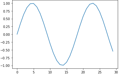
NumPy has a whole host of inbuilt functions that we will explore later, that enable us to add data together, take averages etc..

Pandas

NumPy is great and provides us with a lot of basic needs when it comes to manipulating data, however, it doesn’t always provide us with everything we need.

Pandas significantly enhances NumPy and has gained broad acceptance in the Python community as the data analysis tool for Python. Pandas is built on top of NumPy and so it is dependant on it.

Pandas provides a series object which is akin to a one-dimensional NumPy array but with additional features. Pandas also provides a Dataframe object which is an extension of a NumPy two-dimensional array. One of the key enhancements is the ability to use more general labels for the columns and indexes. This enables us to create, manage and manipulate our data more easily.

In addition to adding data labels and descriptive indices:

It is robust in handling common data formats and missing data
It also allows use of relational-database operations such as joins and merges

Pandas Series objects

Pandas Series objects can be made from Python lists and dicts quite easily:

import pandas as pd

series_from_list = pd.Series([1,2,3,4,5], dtype='float64')
series_from_list

# 0    1.0
# 1    2.0
# 2    3.0
# 3    4.0
# 4    5.0
# dtype: float64

Above we pass in the dtype just like with a NumPy array. 'float64' is the same as np.float64.

A dictionary is quite like a Series and we can use a dict to create a Series:

series_from_dict = pd.Series({0:3, 1:6, 2:9, 3:12, 4:15})
series_from_dict

# 0     3
# 1     6
# 2     9
# 3    12
# 4    15
dtype: int64

All series contain an array that can be retrieved by asking for its values:

series_from_dict.values #=> array([ 3,  6,  9, 12, 15], dtype=int64)

You can also give a series a name. Below we use an array to create a series.

series_from_array = pd.Series(my_array, name='my_array')
series_from_array
# 0    1.0
# 1    2.0
# 2    3.0
# 3    4.0
# 4    5.0
# Name: my_array, dtype: float64

and use .index to obtain its index.

py_dict_series = pd.Series(python_dict)
py_dict_series.index #=> Index(['name', 'realName'], dtype='object')

The dictionary keys have been used as the series Index.

We might also want to change the type of our data and we can perform this change on a scalar, list, tuple, 1-d array, or Pandas Series:

data = pd.to_numeric(series_from_dict)

This will change the data from one type to another. The default return data type is float64 or int64 depending on the data provided.
e.g.

x = pd.Series([1.0, "3", 45])
x = pd.to_numeric(x)
# x
# 0     1.0
# 1     3.0
# 2    45.0
# dtype: float64

Creating a DataFrame from two Series

I have gathered data for the top ten Nintendo Entertainment System game sales from Wikipedia and placed the data into two dictionaries

top_10_NES_sales = {
    'Super Mario Bros.': 40240000, 
    'Duck Hunt': 28300000, 
    'Super Mario Bros. 3': 18000000, 
    'Super Mario Bros. 2': 7460000, 
    'The Legend of Zelda': 6510000, 
    'Tetris': 5580000, 
    'Dr. Mario': 4850000, 
    'Zelda II: The Adventure of Link': 4380000, 
    'Excitebike': 4160000, 
    'Golf':4010000
}  

top_10_NES_years = {
    'Super Mario Bros.': 'September 13, 1985', 
    'Duck Hunt': 'April 21, 1984', 
    'Super Mario Bros. 3': 'October 23, 1988',
    'Super Mario Bros. 2': 'October 9, 1988',
    'The Legend of Zelda': 'February 21, 1986',
    'Tetris': 'November 1989',
    'Dr. Mario': 'July 27, 1990',
    'Zelda II: The Adventure of Link': 'January 14, 1987',
    'Excitebike': 'November 30, 1984',
    'Golf':'May 1, 1984'
 }

First lets make these dictionaries into pandas Series objects and then into a DataFrame object.

top_NES_Sales_series = pd.Series(top_10_NES_sales)
top_NES_years_series = pd.Series(top_10_NES_years)

sales_and_years = pd.DataFrame({'Sales': top_NES_Sales_series, 'Years': top_NES_years_series})

Basic functions in pandas that show us more information about our dataframe.

Display the top five rows of the dataframe:

sales_and_years.head()

Display the last five rows of the dataframe:

sales_and_years.tail()

Display information about the dataframe:

sales_and_years.info()

Returns the dataframe sorted by values in 'Sales' column:

sales_and_years.sort_values(Sales)

Returns the dataframe sorted by value sin the index:

sales_and_years.sort_index()

Extract the index, array and column names using the following attributes:

sales_and_years.index

# Index(['Super Mario Bros.', 'Duck Hunt', 'Super Mario Bros. 3',
#        'Super Mario Bros. 2', 'The Legend of Zelda', 'Tetris', 'Dr. Mario',
#        'Zelda II: The Adventure of Link', 'Excitebike', 'Golf'],
#       dtype='object')

sales_and_years.values

# array([[40240000, 'September 13, 1985'],
#        [28300000, 'April 21, 1984'],
#        [18000000, 'October 23, 1988'],
#        [7460000, 'October 9, 1988'],
#        [6510000, 'February 21, 1986'],
#        [5580000, 'November 1989'],
#        [4850000, 'July 27, 1990'],
#        [4380000, 'January 14, 1987'],
#        [4160000, 'November 30, 1984'],
#        [4010000, 'May 1, 1984']], dtype=object)


sales_and_years.columns #=> Index(['Sales', 'Years'], dtype='object')

You can return a column by indexing the dataframe by its name:

sales_and_years['Years']

Use .iloc to index with numeric indices and .loc for explicit values:

sales_and_years.iloc[0:, 1:]
# Returns all the rows from 0 to the end and all columns from 1 to the end

sales_and_years.loc['Super Mario Bros. 2': 'Excitebike']
# returns all rows and columns with indexes from 'Super Mario Bros. 2' to 'Excitebike'

Import data from a csv using pandas

The Pandas read_csv function is a powerful and versatile tool for reading data and forming a dataframe quickly. You can think of Dataframes like an SQL Table or spreadsheet.
It is customary to import pandas under the alias pd:

import pandas as pd
data = pd.read_csv(‘tips.csv’)

We then call upon Pandas' read_csv method to read a csv file and store that in the variable data.

Returns:

DataFrame
A comma-separated values (csv) file is returned as a two-dimensional data structure with labeled axes.

There is much, much more that can be done using pandas. CSV, NumPy and Pandas are the three basic libraries that will enable you to write backends that can process high amounts of data.

Data Cleaning

Data doesn't always come in the form that is easiest to work with. Real world data can have missing values, or be badly labeled. Sometimes the data just isn't organised or fit for purpose. The process of ensuring our data is fit for purpose is called data cleaning.

It is said that 80% of a Data Scientist's time is spent cleaning the data. The process of Data Cleaning is made easier with Pandas. Pandas has lots of built in functions we can use to help us out. Here are some useful examples.

Dealing With Dates

One common example of values that need cleaning come in the form of dates. Dates can come in many formats (str, numbers, objects), and they can follow different conventions (dd/mm/yy, Month - Day - Year).

Pandas has a convenient tool called to_datetime which deals with such inconsistencies and transforms them to a usable format. Using our dataframe above with the top ten NES sales data we can see that the dates provided are actually strings.

sales_and_years.info()

Below we clean these date values using pd.to_datetime

sales_and_years['Years'] = pd.to_datetime(sales_and_years['Years'])
sales_and_years.info()

# <class 'pandas.core.frame.DataFrame'>
# Index: 10 entries, Super Mario Bros. to Golf
# Data columns (total 2 columns):
#  #   Column  Non-Null Count  Dtype         
# ---  ------  --------------  -----         
#  0   Sales   10 non-null     int64         
#  1   Years   10 non-null     datetime64[ns]
# dtypes: datetime64[ns](1), int64(1)
# memory usage: 560.0+ bytes

Using this method we can transform dates into something very usable as the datetime64 object s Pandas to_datetime will be enough in many occurences where you might need to clean up some datetime values. You can also use the astype method

Dealing With Missing Values

How can we know if our data is missing values? Cast your eyes to the above info print of our top ten NES games data. Among other things the info() method prints Non-Null Count for each column.
Beneath the class the Index info shows us there are 10 entries. So if there are 10 Non-Null values then there shouldn't be any missing values here. To make sure we can use the isnull().sum() method chain:

sales_and_years.isnull().sum()
# Sales    0
# Years    0
# dtype: int64

One of the most common practices of cleaning data is deciding how to deal with missing values:

Do you remove them?
Do you fill them with values that makes sense?
Do you leave them as they are?

The answer depends on the kind of data you are working with. Can you afford to lose data by removing rows or columns with empty values? Or does the missing data tell a story that can be useful in analysis?

If you want to remove them:

data.dropna(x)

If you want to fill with them with a default value:

data.fillna(x)

You are strongly encouraged to look into the various cleaning methods at your disposal using Pandas and NumPy!

Visualising DataFrames

You can use matplotlib for a pandas dataframe for a basic plot eg.

plt.scatter('Years','Sales', data=sales_and_years)

Try annotating the points with annotate:

for i, text in enumerate(sales_and_years.index):
  plt.annotate(text, (sales_and_years['Years'][i], sales_and_years['Sales'][i]))

For more functionality, pandas has its own wrapper around matplotlib. Try out the following and experiment further with the help of the documentation!

sales_and_years.plot('Years', 'Sales', kind='scatter', s=sales_and_years['Sales']/100000, c="Sales", colormap='viridis', title='NES')