04 Getting Started - ge-high-assurance/RACK GitHub Wiki
This page walks you through how to get started with RiB running as an instance on your local machine in a Linux container or virtual machine, using the provided Turnstile example data.
Loading data into RACK (NEW!)
The easiest way to load data is via the RACK UI:
The RACK UI provides a button to load the Turnstile example data.
The legacy process for setting up a local Python environment to launch the command line interface (CLI) and load packages from disk is no longer needed, but still documented below. See Loading with local python.
Another way to load data is via RITE, an Eclipse-based IDE. RITE connects to RACK's triplestore, allows for easy ingestion, integrates with SADL (Semantic Application Design Language) for data model development, and creates ingestion packages. RITE also provides GUI-support for generation of compliance reports to aid in system certification.
RiB's Graphical Interface (SPARQLgraph)
You can access the RiB Welcome page at:
RiB also comes with a graphical user interface called SPARQLgraph, which you can access from the Welcome page or directly through this link:
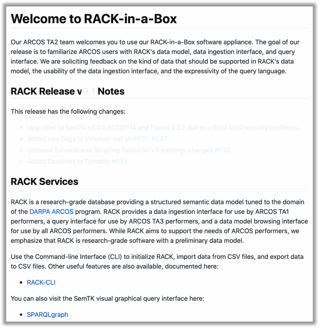
The Welcome page identifies the RACK Release version and release notes, lists RACK services, and provide links to RACK User Guide and Documentation:
From the Welcome page, click on the link SPARQLgraph to bring up the below image. The left hand side is the ontology model pane and the larger pane to the right is the main canvas for building nodegroups.
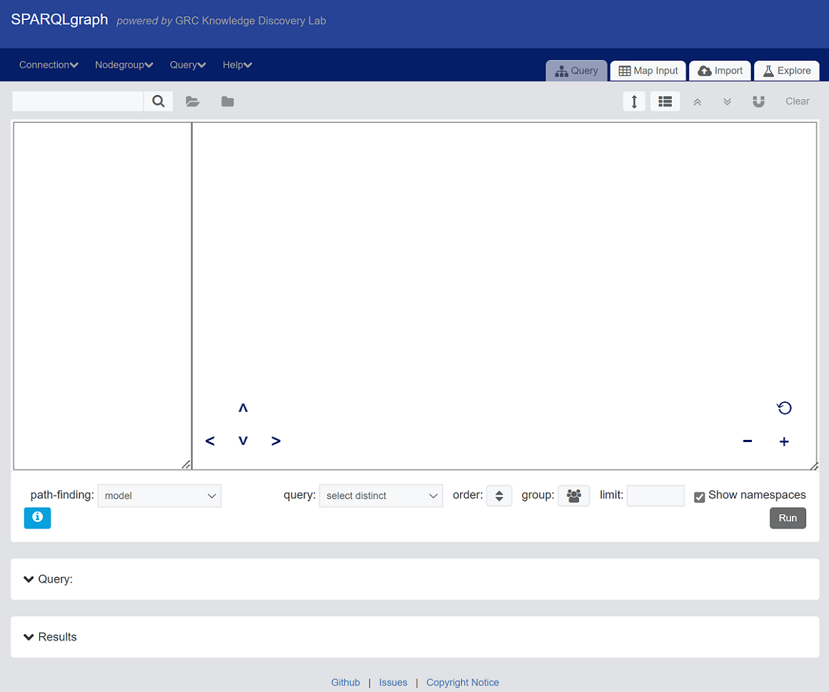
Here's a quick summary of terms you'll want to understand about SPARQLgraph:
- It works on top of a semantic triplestore. In this installation we use the Apache Fuskeki Server.
- It manages "connections" to the triplestore, which include at least one graph that holds the ontology model and one that holds data.
- It manages queries (SELECT, INSERT, and others) through a construct called "nodegroups", which are displayed graphically on the main canvas.
- Nodegroups can be stored in the nodegroup store or as json files.
Create and Save a New Connection
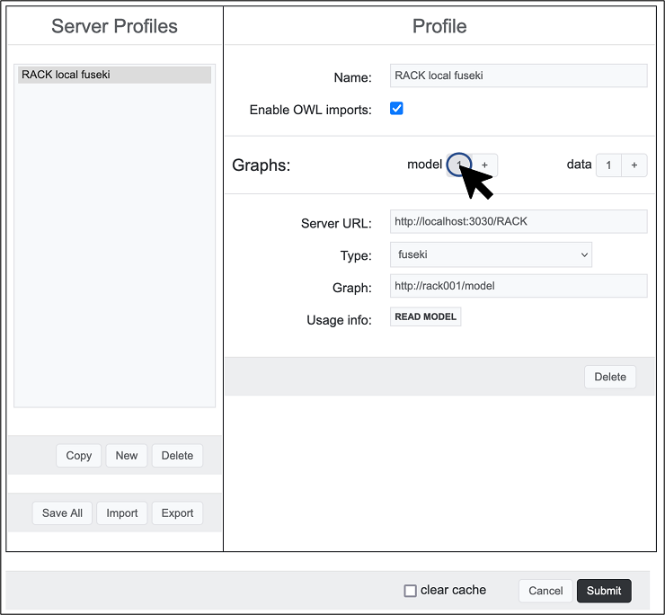
Choose Connection > Load from the menu. A dialog will come up to create a new Server Profile. The fields at the right under Profile is for configuring and building new connections. The most important features of a connection are the graph names and SPARQL endpoint(s) that specify where the ontology model and data are loaded. Click "New" and enter the information so that it looks like this:
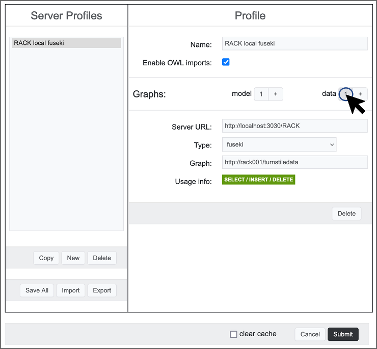
Click the "1" next to "data" and change the "Graph:" entry to
http://rack001/turnstiledata. Hit "Submit".
You have now set up the connection to run queries via SPARQLgraph on the Turnstile data in the next step.
Load a Nodegroup
Let's load a nodegroup from the store.
- choose Nodegroup > Open the store... from the menu.
- click on any entry that starts with "query". This page walks through "query Hazard Structure".
- hit the "Load" button.
- you may be asked to save the connection locally. Hit "Save" to store this connection in your browser for use later.
- if you are prompted with "Nodegroup is from a different SPARQL connection," choose "Keep Current". (This means to use the connection created in the previous step instead of the default connection contained in the nodegroup.)
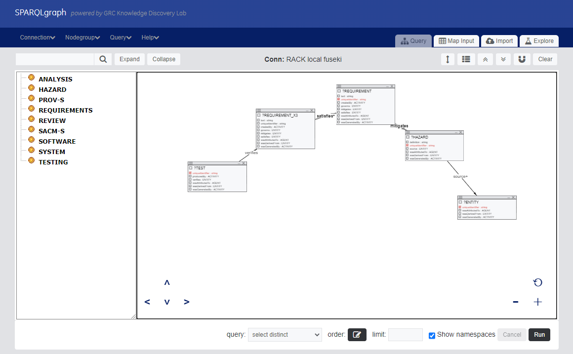
Here are a few things to notice. The left hand side ontology model pane is populated with classes from the model. Clicking a class name will expand it to show its properties and subclasses. (Note: The ontology is subject to change since this is an active research program on DARPA ARCOS. The ontology in the picture may be different from the current release.) To the right, the main canvas displays the nodegroup graphically. The + and - buttons on the bottom-right of the main canvas allows you to zoom in and out; there is also a refresh button to recenter the nodegroup on the canvas. The directional arrows on the bottom-left allows you to pan around the main canvas. In the top-middle, Conn identifies the connection currently being used.
Run the Query
Below the main canvas is the type of query to be run. The default is "select distinct". This is what we will walk through in the next section. Hit "Run". The "query Hazard Structure" contains a runtime constraint which will bring up a dialog that looks like this:
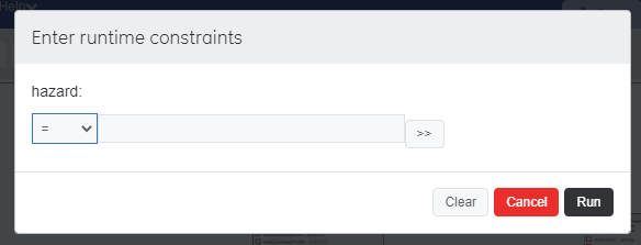
This is allowing you to narrow the values for "hazard". You may ignore this dialog by hitting "Run" or try it out by doing the following:
- keep the default "=" to search only for information about hazards equal to a particular id
- hit the ">>" button to ask SPARQLgraph to generate a query to find all existing values. Choose one.
- hit "Run" to continue
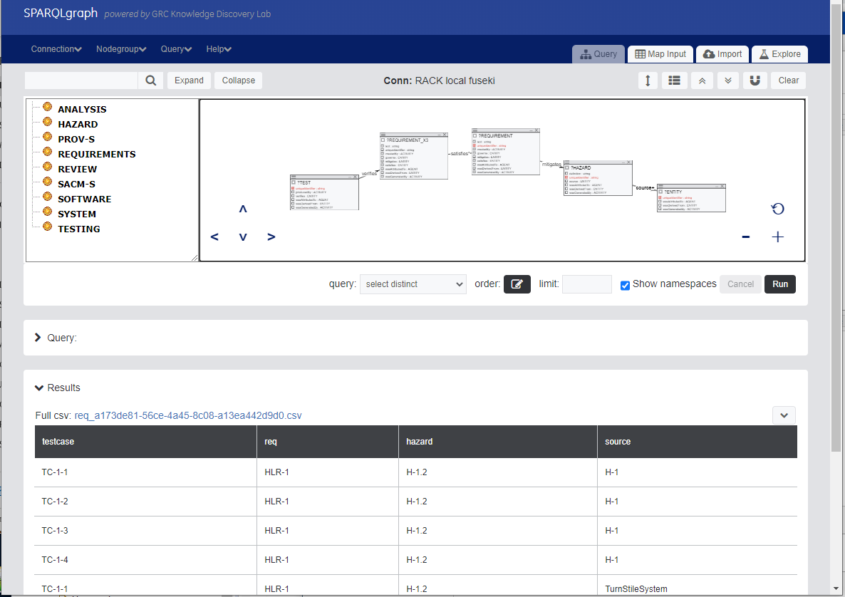
A table of results is returned when running "select distinct" query which contains a row for every unique permutation of values. Results may be saved using the link provided at the top-left of the table, or the drop down at the top-right of the results.
Feel free to try out other queries from the nodegroup store and run them. Descriptions of the preloaded queries are found in the RACK Predefined Queries page.
Queries can also be run using the RACK CLI. Below shows how to run the hazard structure query. The command below specifies the following:
- export data
- the data-graph which is
http://rack001/turnstiledata, same as what was saved in Conn: RACK local fuseki - name of the query json file which is "query Hazard structure.json"
By default the CLI command is looking for localhost running in a
Linux container. See RACK CLI -> Export data
section
for more options such as specifying the base url, setting runtime
constraints, and saving results to a CSV file.
(venv) $ rack data export --data-graph http://rack001/turnstiledata "query Hazard structure"
testcase  req    hazard  source
--------  -----  ------  ------
TC-1-1    HLR-1  H-1.2   H-1
TC-1-2    HLR-1  H-1.2   H-1
TC-1-3    HLR-1  H-1.2   H-1
TC-1-4    HLR-1  H-1.2   H-1
...
Loading with local Python
Optionally, instead of using the new RACK UI (above), you can use the original process of setting up a local Python environment described below. To get started, install the command-line interface (RACK CLI) following the instructions here.
Initialize RiB for the Turnstile Example
Perform the following steps to initialize RiB for the Turnstile
Example. Here the RiB instance is running in a Linux container on
localhost:
$ cd RACK/cli
$ . venv/bin/activate
(venv) $ ./setup-owl.sh
(venv) $ ./setup-turnstile.sh
setup-owl.sh copies files out of the RiB and saves them onto your local hard drive. setup-turnstile.sh loads the data model files and nodegroups for the Turnstile example into RiB.
Load the Turnstile data into RiB
Once initialized, data can be loaded into RiB. We created a sample ingestion package for the Turnstile Example.
(venv) $ cd RACK/Turnstile-Example/Turnstile-IngestionPackage
(venv) $ ./Load-TurnstileData.sh