3 Comparing Time Series - essenius/FitNesseFitSharpSupportFunctions GitHub Wiki

What Is a Time Series?

A time series is a series of data points indexed in time order. It can be represented as tables of data with time stamps, values, and usually an indication of quality (good/bad). Values are typically floating points, but they can also be integers, Booleans or strings. Here is a simple example:

Timestamp	Value	Is Good
1980-01-01T00:00:00.0000000	50	True
1980-01-01T00:01:00.0000000	50	True
1980-01-01T00:02:00.0000000	50	True
1980-01-01T00:03:00.0000000	50.0000000125508	True
1980-01-01T00:04:00.0000000	50.0000000169409	True

Time series are used very often – Sensor outputs are usually sampled into time series data, actuators accept them, simulations and control systems accept and provide them. In general, they provide the inputs and outputs for systems with time dependent behaviors.

Why Do We Want to Compare Time Series Data with FitNesse?

If you design a system, you want to validate that your system delivers the right results. Typically, that happens by providing your system with a certain set of input data, and comparing the results with a reference set of result data. That sounds simpler than it really is. Testing time series data is always a bit tricky, since test runs don’t necessarily provide exactly the same results. The results have to stay within a certain tolerance. And that tolerance is not always the same; it can be relative (a percentage of the range that the values span) or absolute (e.g. 0.001).

Executing these kinds of tests manually is very tedious work, and humans are also not very good at it – it is not easy to identify threshold errors from pages full of data points. So automating these tests makes a lot of sense. We would like to make these tests as re-usable as possible, so we want to use FitNesse to do this, with standard fixtures. The SupportFunctions assembly was extended to provide that capability.

Comparing Floating Point Time Series Data Using CSV Files

Simulation results are often recorded as CSV files, so we want to ensure that we can use those as sources. Let’s have a look how that works. Here is how you specify a simple test.

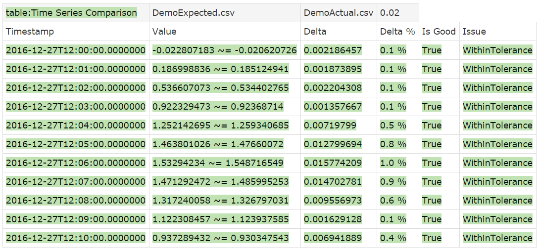
!|table:Time Series Comparison|DemoExpected.csv|DemoActual.csv|0.02|

We use a Table table called Time Series Comparison. Parameters are the expected time series, the actual time series and the tolerance. So in this case, FitNesse will read DemoExpected.csv, and compare it to DemoActual.csv. For the values, it will take a tolerance of 0.02, i.e. if the actual value is within 0.02 of the expected value (higher or lower), the test for that value will pass. The test data also has an Is Good column (Boolean result: true/false) which also needs to be validated.

Here is DemoExpected.csv (and DemoActual.csv looks similar)

Timestamp,Value,IsGood
2016-12-27T12:00:00.0000000,-0.020620726,TRUE
2016-12-27T12:01:00.0000000,0.185124941,TRUE
2016-12-27T12:02:00.0000000,0.534402765,TRUE
2016-12-27T12:03:00.0000000,0.92368714,TRUE
2016-12-27T12:04:00.0000000,1.259340685,TRUE
2016-12-27T12:05:00.0000000,1.47660072,TRUE
2016-12-27T12:06:00.0000000,1.548716549,TRUE
2016-12-27T12:07:00.0000000,1.485995253,TRUE
2016-12-27T12:08:00.0000000,1.326797031,TRUE
2016-12-27T12:09:00.0000000,1.123937585,TRUE
2016-12-27T12:10:00.0000000,0.930347543,TRUE

The screen shot shows the result. We are all good. The notation ~= means “equal within tolerance”. The Delta column show the absolute difference between expected and actual values. The Delta % column shows the relative difference with the time series range (i.e. the difference between the largest and the smallest value in the series). The last column describes the outcome of the comparison. Here everything is WithinTolerance, which means that the difference was less than the specified tolerance.

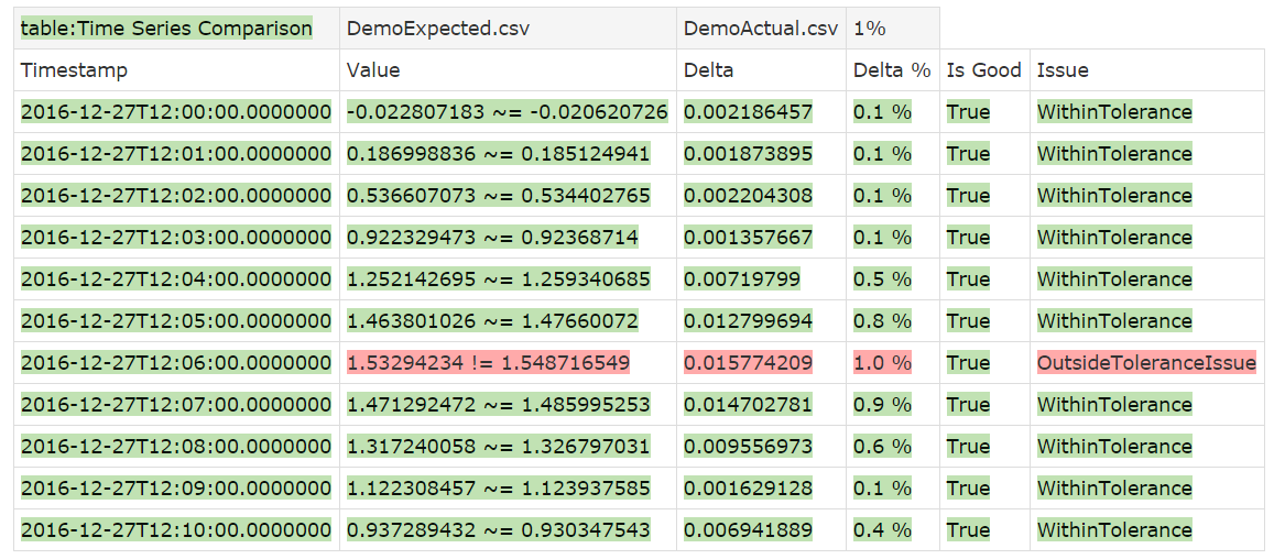
Instead of an absolute value for the tolerance, we can also specify a percentage, say 1%.

!|table:Time Series Comparison|DemoExpected.csv|DemoActual.csv|1%|

The result shows that now one value falls just outside of the tolerance.

You will have noticed that a lot of significant digits are displayed. It can clutter the view if the actual precision of the data is lower than the displayed precision. That is why it’s also possible to specify the desired precision of the tolerance, which will then also be used to determine the display precision of the expected and actual values. The following specification will require the absolute tolerance to be rounded to 3 significant digits, and the values and deltas will be aligned to the precision that leads to:

!|table:Time Series Comparison|DemoExpected.csv|DemoActual.csv|1%:3|

The result shows that indeed the values and delta now have 4 fractional digits, which aligns with 3 significant digits for the absolute tolerance (which is not shown but is 0.0157 since the range of the time series is 1.569337275). The actual and expected values now show the same precision. The comparison is done with the non-rounded expected and actual values, against the (rounded) tolerance.

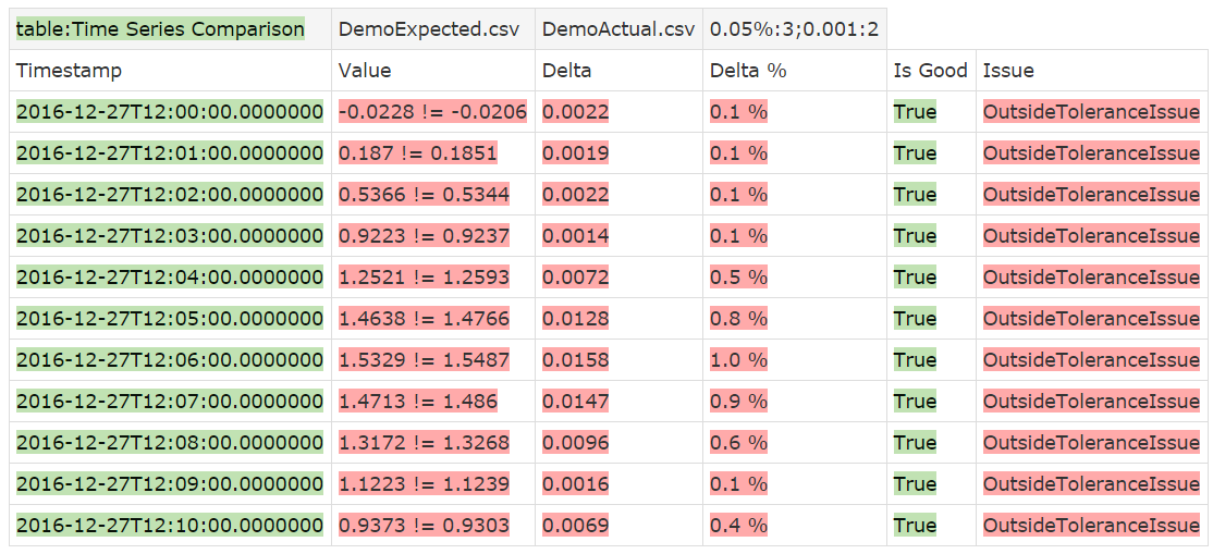
Sometimes you can’t predict the data range in advance, and you want to specify a minimal absolute tolerance regardless of what the relative tolerance results in. For example, suppose we want to have a tolerance of 1% of the expected range, but it should be no smaller than 0.001. You can specify multiple tolerances by separating them with a semicolon (;). The maximum tolerance will then be applied.

!|table:Time Series Comparison|DemoExpected.csv|DemoActual.csv|1%:3;0.001:2|

We specify the significant digits for the absolute tolerance as well, so the comparison results are also displayed rounded if the absolute tolerance is used. If you run it like this, you will see no difference since 0.0157 is larger than 0.001, so the used tolerance is 0.0157. But if you e.g. change the percentage to 0.05%, then the absolute value kicks in, and now none of the values match. Notice how the precision is still 4 digits. That’s because the tolerance value is actually 0.0010 (two significant digits).

The default for tolerance is 0. Because of the way floating point values are stored, it is unlikely that a delta will be exactly 0. So, you should always define a tolerance for floating points. You could use epsilon to get the smallest double value above 0. But do note that when using epsilon (requiring a precision of over 300 digits after the decimal point) you can’t use rounding, as that doesn’t work with precisions over 15 digits. If you try, it will be ignored.

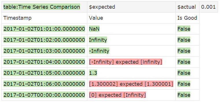
You can also use the special cases NaN (not a number), Infinity and -Infinity as valid floating-point values.

The casing is important here. If you spell them differently, e.g. not capitalizing the first letter (infinity) then the value will be interpreted as a string, not a floating point. If it occurs in the expected values, the time series comparison will be done using string comparison. That is shown in the example below. In the 4th data point, Infinity is misspelled as infinity. You will see that the tolerance is no longer showing in the Value header, indicating that we are not executing a floating-point comparison. Also, the numerical comparison in the 6th point does not pass, since the strings are not equal.

Comparing Non-Floating Point Time Series

So far, we used floating point (double) values for the comparison. However, the fixture can also deal with integers, long integers, Booleans and strings. For integers and long integers, you can also specify a tolerance. This can e.g. be useful for very large numbers such as ticks, where quite large tolerances could be appropriate, given that there are 10,000 ticks in a millisecond. Relative tolerances for (long) integers are rounded to the nearest integer. For Boolean and string values, the tolerance setting is ignored and comparison is always exact. The fixture determines which data type to use for the comparison by examining the expected data:

1. If all data points are integers, then an integer comparison is done.
2. If we have a mix of integers and long integers, then a long integer comparison is done.
3. With a mix of integers, longs, and double (floating point), a double comparison is done.
4. If all values are Booleans (evaluate to true or false) then a Boolean comparison is done.
5. In all other cases, a string evaluation is done.

Specifying Time Series in FitNesse

It would be useful if we could specify the expected data directly in FitNesse besides relying on CSV files. To support that, the Support Functions assembly has a Time Series fixture with a Decision table interface. To make that work, we need a reference to the table that we can pass to the Time Series Comparison fixture. A trick to do that is the following:

|Script    |Time Series|
|$expected=|get fixture|

Basically, all this does is creating a TimeSeries object, and passing that to the $expected symbol. Now you can use this reference in a decision table to create a data set:

!|decision:$expected              |
|Timestamp          |value|is good|
|2014-01-01T00:00:00|Hi1  |True   |
|2014-01-01T00:00:01|Hi3  |True   |
|2014-01-01T00:00:02|Hi4  |True   |
|2014-01-01T00:00:03|Hi5  |True   |
|2014-01-01T00:00:04|Hi6  |False  |

To complete the example, we create an actual time series table the same way, and then we run the comparison. Now, instead of the file name, we use the symbols to identify the time series data.

|Script  |Time Series|
|$actual=|get fixture|

!|decision:$actual                  |
|Timestamp            |value|is good|
|2014-01-01T00:00:00  |Hi2  |False  |
|2014-01-01T00:00:01  |Hi3  |True   |
|2014-01-01T00:00:03  |Hi4  |True   |
|2014-01-01T00:00:04  |Hi6  |True   |
|2014-01-01T00:00:04.5|Hi4  |True   |

!|table:Time Series Comparison|$expected|$actual|

We’ll discuss the outcome of this comparison in the next section.

Exact Comparisons and Data Point Mismatches

Here is the result of the test case that we defined in the previous section:

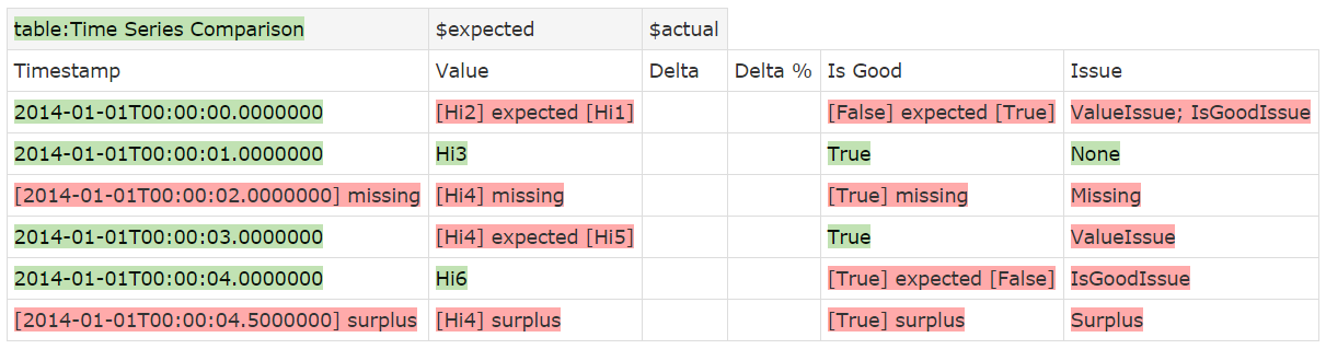
To avoid ambiguity, test results will always show the .Net DateTime roundtrip format, even if the input data uses a different format. If the fixture can convert the input data to a valid DateTime object, it will accept it, adding default data if it needs to. So, for example, if you only specify times, then the current date will be added. You can also use a long integer as the timestamp; in that case the value will be interpreted as a .Net Ticks value (see section 8.2). For the comparison, all timestamps will be converted into a DateTime object.

This example also shows what happens if there are data mismatches with exact matching: the default FitNesse notation of [actual] expected [expected] is used. This works for both the Value and the Is Good column. If a data point in the expected set can’t be matched, then the Timestamp, Value, Is Good and Issue fields are failed and missing is added, just like with FitNesse’s query interface. Likewise, if an actual data point cannot be matched to an expected data point, then the fields are failed and surplus is added.

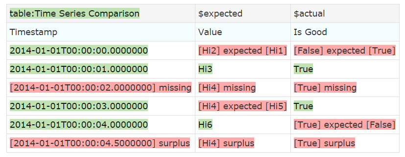
You will notice that the Delta and Delta % columns are superfluous here as we don’t have numerical comparisons. You may also not necessarily be interested in the Issue column. You can show only the columns you want in the following way:

!|table:Time Series Comparison|$expected|$actual|
|Timestamp|Value|Is Good|

This is the result:

Using CSV Files with Different Column Names

You don’t always entirely control the way that your test data is provided. CSV is quite common, but it is not so likely that the data will use the exact same column names. Therefore, it is possible to override the standard column names used to identify the data you need. There are two ways of doing that. We will show both ways. The first one uses the same trick we saw to define Time Series data; the other one shows a short-hand way. We use one table for both expected and actual data. The structure is as follows:

Timestamp,ExpectedValue,ExpectedQuality,ActualValue,ActualQuality
1980-01-01T00:00:00.0000000,50,True,50,True
1980-01-01T00:01:00.0000000,50,True,50,True
1980-01-01T00:02:00.0000000,50,True,50,True
1980-01-01T00:03:00.0000000,50.0000000414593,True,50.0000000125508,True
1980-01-01T00:04:00.0000000,50.0000000158153,True,50.0000000169409,True
1980-01-01T00:05:00.0000000,50.0000000104932,True,50.0000000164372,False
1980-01-01T00:06:00.0000000,49.9752835096486,True,49.9739350539787,True

We use a variable to hold the file name, as we’re using it more than once. Then we define a time series object using a script table, and we use the Set Value Column and Set Is Good Column commands to overrule which column names identify the value and the is good columns. Then we put the object into a symbol $expectedSeries so we can use it in the time series comparison.

The other way is putting the desired column names next to the file name in the comparison table, separated by hash (#) symbols. That is shown for the actual time series data. If you don’t want to change the column name to use, leave it blank (we could have done that here with Timestamp).

!define CombinedCsv {!-CsvTestDataCombined.csv-!}

!|script           |Time Series|${CombinedCsv}|
|Set Is Good Column|ExpectedQuality           |
|Set Value Column  |ExpectedValue             |
|$expectedSeries=  |get fixture               |

|table:time series comparison|$expectedSeries|${CombinedCsv}#Timestamp#ActualValue#ActualQuality|0.0013:4|

Here is the outcome:

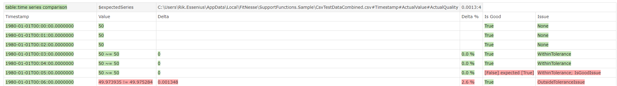
The first three lines show another feature that may not be immediately obvious. If the values can be exactly matched, then the approximate match notation is not used. So the first three values are exactly equal, and the next 3 are equal within the tolerance (and even within the precision). This feature also ensures that double NaN and Infinity values can be matched.

Why Use a Table Table for the Comparison Instead of a Query Table?

You might think that the query table is ideally suited to support the time series comparison. Then you could specify the expected values in the query table, and let FitNesse handle the comparison. However, that would be less flexible, as then you could not specify the expected values in a CSV file. Furthermore, the comparison would require a custom comparator in FitNesse, which would imply more configuration work for FitNesse. Also, we couldn’t customize the value column header to show the tolerance. Using a Table Table seems the more logical choice, even if it means we need to replicate some FitNesse comparison functionality in the fixture code.

Graphical Representations of the comparison

People tend to be much better at interpreting charts than rows of data. So that is why it is possible to include a graphical representation of the comparison if required. That is provided via a script table interface. You don’t need to run the table table before showing the chart; if the comparison hasn’t been done before it will be done automatically. To ensure that we can still automatically pass/fail, we also have two summary functions: Failure Count and Point Count. The first one returns the number of data points having mismatches, and the second returns the total number of data points tested.

To make this work, there is one thing you need to do manually, and that is copying libSkiaSharp.dll from runtimes\win-x64 (change for your machine type if needed) to the net5.0 folder.

Going back to one of the previous examples, here is how you create a test with a graphical result:

!|script:Time Series Comparison|${folder}\DemoExpected.csv|${folder}\DemoActual.csv|0.5%:3;0.01|
|check                         |failure count             |3                                   |
|check                         |point count               |>0                                  |
|check                         |base timestamp            |2016-12-27T12:00:00                 |

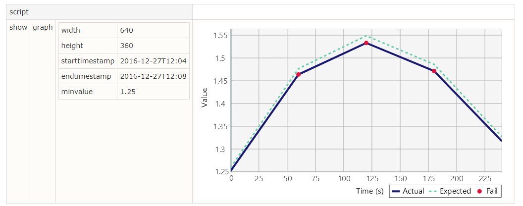
|script                                                                                                                   |
|show|graph|!{width:640, height:360, starttimestamp:!-2016-12-27T12:04-!,endtimestamp:!-2016-12-27T12:08-!, minvalue:1.25}|

The red dots show test failures. Indeed, there are 3 dots, and the failure count is 3.

As the example shows, you can have FitNesse check for success by just including tests whether the failure count is 0 and the point count is greater than 0. And for these functions also, if the comparison hasn’t been done already it will be done before returning the result.

You might notice that the script table has been split: we end a table and start a next one without a name. That will simply continue using the same fixture as the previous table. This is an easy way to force resizing different parts of the table so it won’t spread out horizontally so much. To show the point, here is what the result would look like if you use one table:

If you want to have a closer look at certain parts of the graph, you can do that too. Suppose we want to have a closer look at the errors. First, we find out the base timestamp (i.e. the timestamp of the first data point), and then we specify an interval via starttimestamp and endtimestamp. We can also specify Y axis limits via minvalue and maxvalue:

Notice how the X axis unit has now moved from minutes to seconds. The scale will automatically adjust from milliseconds to seconds, minutes, hours or days based on the interval being displayed. The script for this is:

|script                                                                                                     |
|show|graph|!{width:640, height:360, starttime:!-2016-12-27T12:04-!, endtime:!-2016-12-27T12:08-!, min:1.25}|

We use the !- -! notation in the start and end times to make sure that FitNesse doesn’t interpret the colons in the timestamp as dictionary separators.