RNA‐seq Analysis Recipe - epigen/MrBiomics GitHub Wiki
The RNA-seq Analysis Recipe takes you from publicly available raw uBAM files derived from a bulk RNA-seq experiment to enrichment analysis results of differentially expressed genes while providing genome browser tracks for quality control, comprehensive reporting on processing and unsupervised analyses. Specifically, it walks you through the workflow specified in workflow/rules/CorcesRNA.smk.
Note
Before you begin, please review our general guide on How to use Recipes and switch your browser to light mode otherwise you might experience reading difficulties with some of the figures.
Tip
Explore the full interactive report:
This wiki page highlights key analyses, decisions and results. For more results explore the complete interactive Snakemake report, where all results specific to this recipe are prefixed with CorcesRNA_*.
In this tutorial, we want to identify the gene signatures and biological pathways that characterize 13 distinct cell types within the human hematopoietic system. We will re-analyze a published RNA-seq dataset from Corces et al. (2016), which we call CorcesRNA, to demonstrate a reproducible and modular analysis workflow. Below we provide a complete guide for analyzing this dataset, starting from retrieving raw sequence files and culminating in the identification of cell-type-specific gene signatures, enrichments and the computational reconstruction of the hematopoietic lineage.
Tip
This recipe is also ideal for pseudobulk scRNA-seq analysis!
While this tutorial uses a bulk RNA-seq dataset, the workflow is perfectly suited for analyzing pseudobulked single-cell RNA-seq (scRNA-seq) data. Analyzing pseudobulk samples, e.g., by aggregating counts for each cell type, condition and patient, is a statistically robust method to handle inter-individual variability and avoid the false positives common in single-cell-level analyses. You can then use the processing (with spilterlize_integrate), powerful linear modeling (with dea_limma) and enrichment analysis (enrichment_analysis) described here to analyze complex experimental designs with many covariates (e.g., ~ cell_type + condition + patient).
Important
Why: Identifying gene expression signatures that characterize distinct cell types or biological states is a cornerstone of modern molecular biology. This process is fundamental for understanding complex systems like development, immunity, and disease. Furthermore, the resulting genes can serve in basic research as markers or in translational research for diagnostics, therapeutic targeting, or engineering new cellular functions.
At the end of this tutorial, you will have a clear understanding of the scientific goals and the biological context of RNA-seq analysis.
To achieve our goal, we combine a series of interconnected MrBiomics Modules into a Recipe. Each module performs a specific task, creating a powerful and flexible analysis pipeline. The overall strategy is to first process the raw data, perform quality control, identify differentially expressed genes for each cell type, interpret these gene lists biologically, and finally, reconstruct the hematopoietic lineage computationally using a custom rule. The recipe is structured as follows(*):
flowchart LR;
    fetch_ngs-->rnaseq_pipeline;
    rnaseq_pipeline-->genome_tracks;
    rnaseq_pipeline-->spilterlize_integrate;
    spilterlize_integrate-->unsupervised_analysis;
    spilterlize_integrate-->dea_limma;
    dea_limma-->enrichment_analysis;
    spilterlize_integrate-->crossprediction_analysis;
We use the following MrBiomics modules and one custom script:
- Fetch NGS: Downloads public bulk RNA-seq data.
- RNA-seq pipeline: Quantifies gene expression to produce count matrices and annotations.
- Genome Browser Track Visualization: Creates genome tracks for visual quality control and analysis of genomic regions of interest.
- Split, Filter, Normalize & Integrate: Filters, normalizes, and integrates data for downstream analysis.
- Unsupervised Analysis: Explores data structure and sample similarity using PCA and UMAP.
- Differential Analysis with limma: Identifies statistically significant genes between cell types using linear modeling.
- Enrichment Analysis: Provides biomedical interpretation of differential analysis results using prior knowledge.
- Crossprediction analysis: A custom script to computationally reconstruct human hematopoietic lineage.
Templates of corresponding Methods sections for a scientific publication can be found in each module's README.
Note
Checkpoint: You have reviewed the function of each module by visiting their respective GitHub pages. You should have a conceptual map of how raw data is transformed into biological insight.
(*)The Recipe's real rulegraph visualizes all steps and their dependencies. While its scale may seem daunting, the rulegraph powerfully illustrates the complexity and sheer number of analytical steps that are fully automated by this Recipe, offering a direct appreciation for the workflow's depth and transparency. It is best treated as a navigable blueprint: you can zoom in to trace the flow of data and dependencies, providing a detailed, step-by-step understanding of the entire workflow.
A key advantage of this recipe is that it requires no custom coding. The entire analysis is orchestrated through Snakemake using pre-existing modules and one custom script, with all parameters controlled by simple configuration files. This approach ensures maximum reproducibility and accessibility for users with varying levels of expertise.
Important
Prerequisites: The total disk space required is approximately 600GB (including temporary files), and the workflow takes ~2-3 hours to run on a high-performance computing (HPC) cluster. Experience in Snakemake workflow usage is highly recommended.
The main components are:
-
Main configuration (
config/config.yaml): The central file that points to all other analysis configurations in the sectionCorcesRNA. -
Dataset/analysis-specific files (
config/CorcesRNA/): A dedicated directory containing all annotation and configuration files for theCorcesRNAanalysis. This modular organization makes it easy to adapt the recipe for other datasets. -
Workflow logic (
workflow/rules/CorcesRNA.smk): The dedicated Snakemake workflow file that defines the rules and connects the modules. -
Custom script (
workflow/scripts/crossprediction.py): A Python script for lineage reconstruction using crossprediction
Tip
Why: Separating the code (modules) from the configuration (YAML/CSV files) is a core principle of reproducible research (separation of concerns). It allows anyone to re-run the exact analysis by simply using the same configuration files, and it allows others to easily apply the same workflow to new data by creating a new set of configuration files.
Note
Checkpoint: You have located all the configuration, annotation and Snakemake files mentioned above within the project structure.
This section details each stage of the analysis, explaining the methods, key decisions, and results. We are re-analyzing bulk RNA-seq data from Corces et al. Lineage-specific and single-cell chromatin accessibility charts human hematopoiesis and leukemia evolution. (2016) Nature Genetics containing 49 healthy donor samples across 13 cell types of human hematopoiesis.
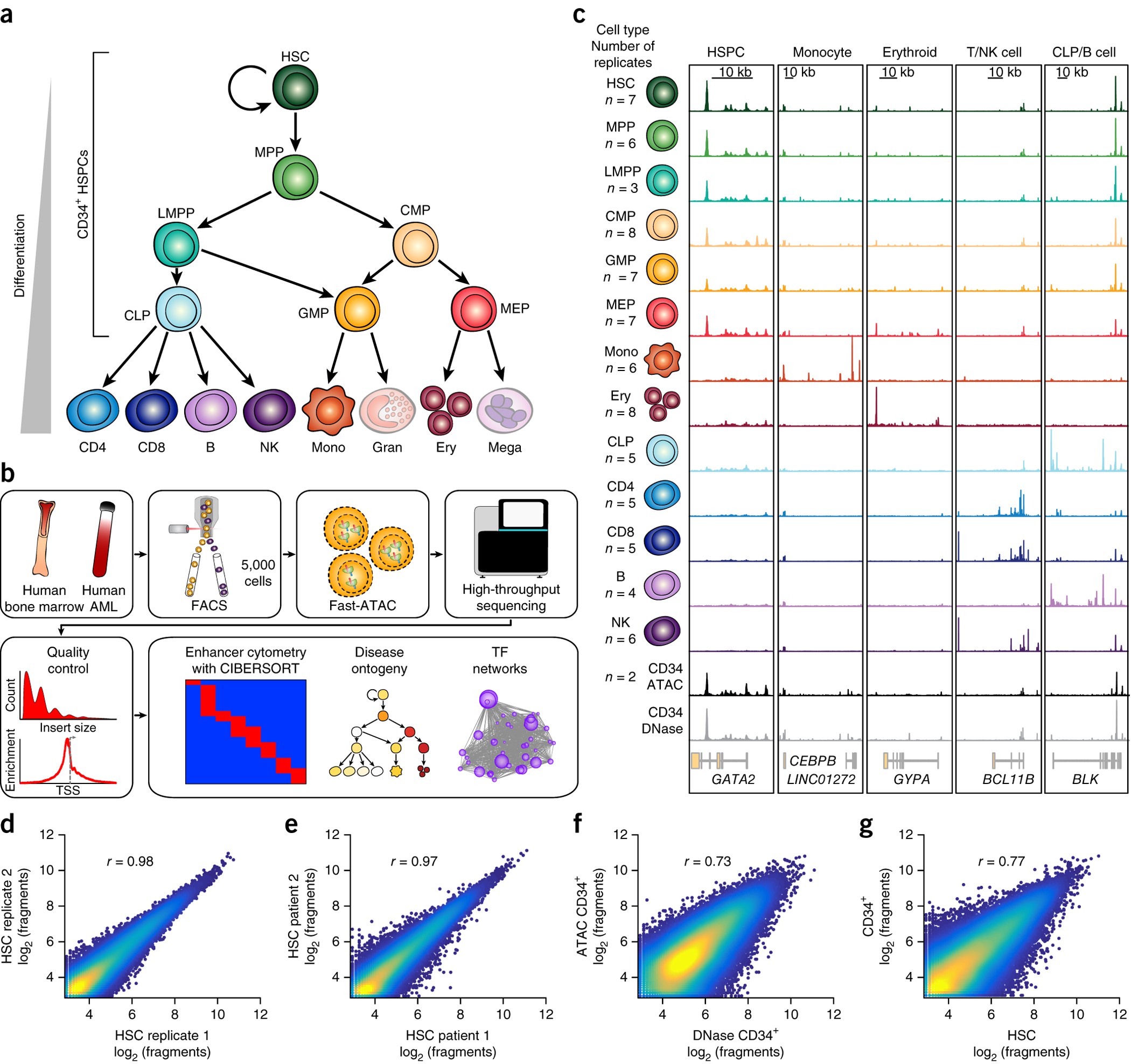
Figure 1 from Corces et al. introducing the dataset and underlying biology
Note
Checkpoint: You have looked at the original Corces et al. paper and understand the basic principles of human hematopoiesis.
4.1 • Data Acquisition with fetch_ngs
Configuration: config/CorcesRNA/CorcesRNA_fetch_ngs_config.yaml
Tip
How to execute each step: Each step of this recipe is performed by a dedicated MrBiomics Module. For detailed instructions on its features and usage, please refer to the module's own documentation page always linked in the headline of the section.
We begin by downloading the raw sequencing data for the CorcesRNA project from the Gene Expression Omnibus (GEO) under accession GSE74246 SuperSeries for unstranded RNA. We first fetch the metadata for all samples in the SuperSeries (using the metadata_only feature) but selectively download only the 49 runs corresponding to healthy donors, excluding leukemia samples (i.e., configuring the selected samples based on the downloaded metadata). The data is downloaded and converted to unaligned BAM (uBAM) files.
Note
Checkpoint: The results/CorcesRNA/fetch_ngs/ directory contains a metadata.csv and 49 subdirectories, each with a *.bam file.
4.2 • Read Alignment and Quantification with rnaseq_pipeline
Configuration: config/CorcesRNA/CorcesRNA_rnaseq_pipeline_config.yaml
Annotation: config/CorcesRNA/CorcesRNA_rnaseq_pipeline_annotation.csv
Using the generated metadata file and the 49 uBAM files, we quantify gene expression. The rnaseq_pipeline module aligns the reads to the human genome (GRCh38) using the STAR aligner and quantifies read counts per gene. This process generates a count matrix (genes × samples), which is the primary input for all subsequent analyses. It also produces comprehensive gene and sample annotation files enriched with quality control (QC) metrics.
During a QC step, sample Mono_7256 (SRR2753109) caused an error because all its reads had a quality score of 0 and were filtered out by fastp. Therefore, we removed it from the sample annotation sheet and thereby our analysis. This leaves a final dataset of 48 high-quality samples for downstream analysis.
→ samtools view results/CorcesRNA/fetch_ngs/SRR2753109/SRR2753109.bam | head -n 5
SRR2753109.1    77      *       0       0       *       *       0       0       AGCTCNCCCCCCACTACNTAAAAAATCCCATACATATACCTGCCCCCCTCACACCCAATTGGCCNNCTCTATCGNC !!!!!!!!!!!!!!!!!!!!!!!!!!!!!!!!!!!!!!!!!!!!!!!!!!!!!!!!!!!!!!!!!!!!!!!!!!!!    RG:Z:A
SRR2753109.1    141     *       0       0       *       *       0       0       NNNNNNNNNNNNNNNNNNNNNNNNNNNCTTNN        !!!!!!!!!!!!!!!!!!!!!!!!!!!!!!!!     RG:Z:A
SRR2753109.10   77      *       0       0       *       *       0       0       AACTTNTTCCGTTGGTCAAGTTATTGGATCAATTGAGTATAGTAGTTCGCTTTGACTGGTGAAGTCTTAGCATGT  !!!!!!!!!!!!!!!!!!!!!!!!!!!!!!!!!!!!!!!!!!!!!!!!!!!!!!!!!!!!!!!!!!!!!!!!!!!     RG:Z:A
SRR2753109.10   141     *       0       0       *       *       0       0       NNNNNTANANNNNACNAGTGANNNNGNCCTGCNNNNNNNNNNNNNNNNNNNNNNNNNNNNNNNNNNNNNNNNNNNN !!!!!!!!!!!!!!!!!!!!!!!!!!!!!!!!!!!!!!!!!!!!!!!!!!!!!!!!!!!!!!!!!!!!!!!!!!!!    RG:Z:A
SRR2753109.100  77      *       0       0       *       *       0       0       CCAATTACACAAATAAAGTATAGGCGAAAGAAATTGAAACCTGGGGCAAAAGATTTAGTACCGCATGGTAAAGATG !!!!!!!!!!!!!!!!!!!!!!!!!!!!!!!!!!!!!!!!!!!!!!!!!!!!!!!!!!!!!!!!!!!!!!!!!!!!    RG:Z:A
A MultiQC report and a heatmap visualizing QC metrics with matching metadata of all samples are generated, aggregating QC metrics from all tools. Given that this is a re-analysis of a published, high-quality dataset, all 48 samples pass our standard QC thresholds (e.g., >70% alignment rate, >10M mapped reads), so no further samples are removed. Clustering on QC metrics clearly separates samples by donor, revealing a donor-specific batch effect that must be accounted for downstream.
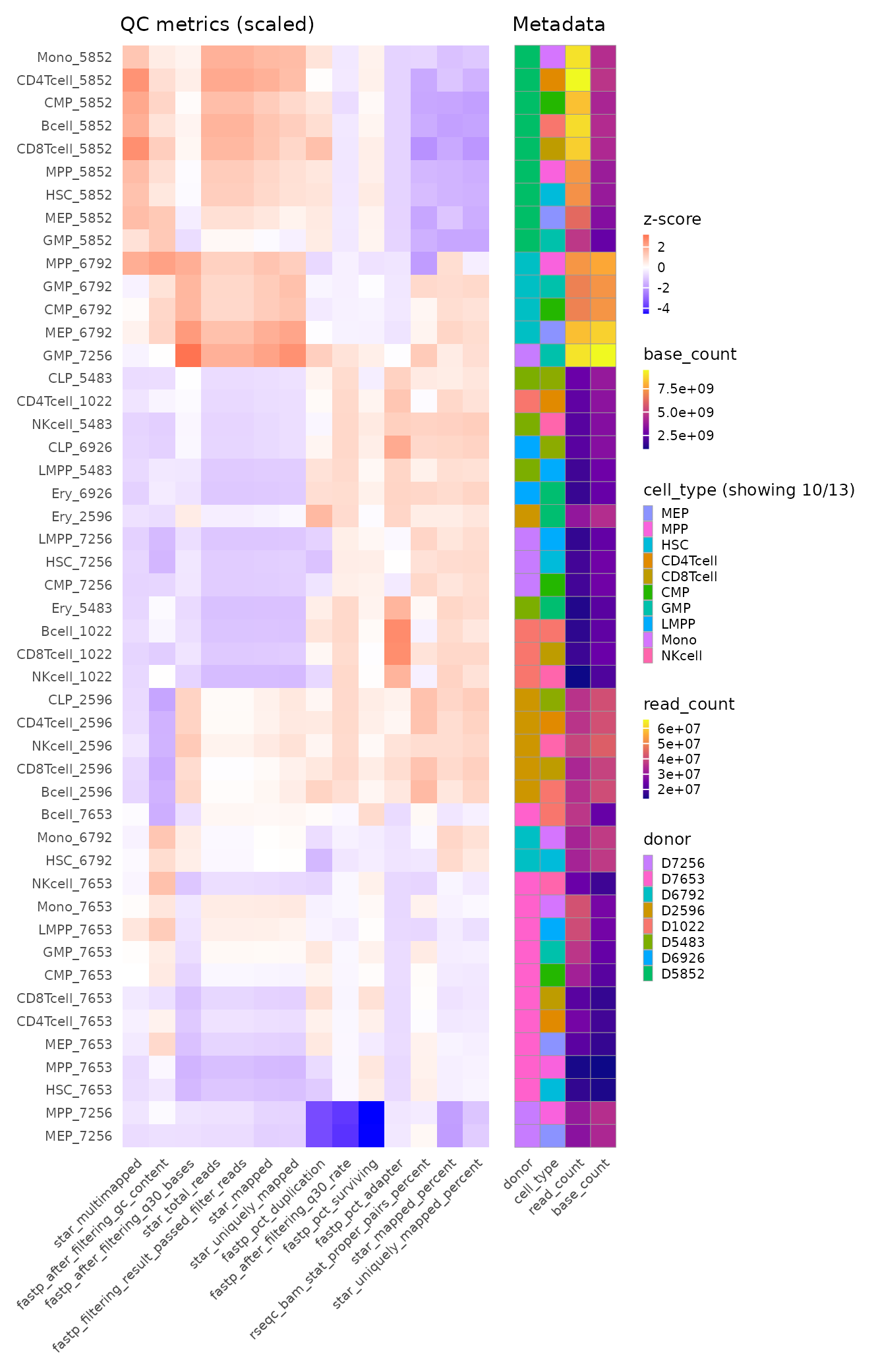
Hierarchically clustered QC heatmap with matching metadata annotation
Note
Checkpoint: The results/CorcesRNA/rnaseq_pipeline/counts/ directory contains three key files: counts.csv, sample_annotation.csv, and gene_annotation.csv. The MultiQC report in results/CorcesRNA/rnaseq_pipeline/report/ shows consistent, high-quality metrics across all 48 samples. The removed sample SRR2753109 is absent from the sample annotation file and results.
4.3 • Visual Quality Control with genome_tracks
Configuration: config/CorcesRNA/CorcesRNA_genome_tracks_config.yaml
Annotation: config/CorcesRNA/CorcesRNA_genome_tracks_annotation.csv
For an intuitive quality check, we visualize the aligned data as genome browser tracks. We use the genome_tracks module to generate coverage plots for 22 known hematopoietic marker genes (e.g., CD34 for stem cells, MS4A1-aka CD20-for B-cells). Samples are grouped by cell type, so all replicates for a given cell type are merged into a single track.
This visualization serves as a critical sanity check. For example, we expect to see high signal for the MS4A1 gene in the Bcell track and low signal elsewhere. Confirming these known patterns gives us confidence in the cell type labels and the overall quality of our data.
| CD34 (stem-ness) | MS4A1 (aka CD20; B cells) |
|---|---|
 |
 |
Note
Checkpoint: The directory results/CorcesRNA/genome_tracks/tracks/ contains PDF/PNG images for all 22 marker genes. Visual inspection confirms that expression patterns align with known hematopoietic biology.
4.4 • Filtering, Normalization and Integration with spilterlize_integrate
Configuration: config/CorcesRNA/CorcesRNA_spilterlize_integrate_config.yaml
Annotation: config/CorcesRNA/CorcesRNA_spilterlize_integrate_annotation.csv
Raw counts require filtering of non-expressed genes, normalization to account for technical artifacts like library size or gene length/GC-content and integration to address potential batch effects. The spilterlize_integrate module is used for these crucial pre-processing steps.
Gene filtering is applied using the default settings. A key diagnostic, the mean-variance plot, subsequently reveals no upward trend among lowly expressed genes, confirming that the filtering effectively removes noise prior to normalization, a critical prerequisite for reliable linear modeling downstream.
Our confounding factor analysis (CFA) reveals a significant association between Principal Component 1 (PC1) and sample GC content. To address this, we apply Conditional Quantile Normalization (CQN), a method specifically designed to correct for both GC content and gene length biases.
Tip
Why CQN? Standard normalization methods like CPM or TMM correct for library size but not for feature-specific biases. The CFA plot clearly showed a GC-content bias, which can lead to false results. CQN addresses this directly, leading to a cleaner signal for biological discovery.
After CQN, we use limma's removeBatchEffect function to integrate the data, modeling cell_type as the variable of interest and removing the donor effect as an unwanted batch covariate. The post-integration CFA confirms that cell_type is now the dominant source of variation.
Important
Always inspect diagnostic plots after each step: After every data transformation—be it splitting, filtering, normalization, or integration—you must inspect the generated diagnostic plots in the report. Pay special attention to the mean-variance plots, PCA plots, and the Confounding Factor Analysis (CFA). This is the only way to visually confirm the impact of each method and to make informed decisions for subsequent analyses.
filtered |
normCQN_integrated |
|---|---|
 |
 |
filtered |
normCQN_integrated |
|---|---|
 |
 |
Note
Checkpoint: All configured processing step result files in results/CorcesRNA/spilterlize_integrate/all/ have been generated. The associated diagnostic plots show that sample distributions are well-aligned and that confounding factors, such as the GC-content or donor effect have been successfully mitigated.
4.5 • Exploratory Data Analysis with unsupervised_analysis
Configuration: config/CorcesRNA/CorcesRNA_unsupervised_analysis_config.yaml
Annotation: config/CorcesRNA/CorcesRNA_unsupervised_analysis_annotation.csv
With a clean, normalized data matrix, we use the unsupervised_analysis module to explore its structure. Principal Component Analysis (PCA) and Uniform Manifold Approximation and Projection (UMAP) are applied to visualize the relationships between samples.
The resulting plots show that samples cluster cleanly by their annotated cell type. We observe that progenitor cells (e.g., HSC, MPP) cluster closely together, while more differentiated cell types (e.g., Erythrocytes, B-cells) form distinct, separate groups. This confirms that our processing has preserved the underlying biological structure. Additionally, we can compare our results to the published results shown here. For efficiency in later steps, we have also generated in the previous step a dataset containing only the top 10% highly variable features (HVFs), which sufficiently capture the cell type characteristics.
normCQN_integrated |
normCQN_integrated_HVF |
|---|---|
 |
 |
normCQN_integrated |
normCQN_integrated_HVF |
|---|---|
 |
 |
Having confirmed that the CQN normalized data provides the clearest biological signal, with samples clustering distinctly by cell type, we will use this dataset for the next step: identifying cell-type-specific gene signatures. The previously observed donor variability will be explicitly modeled as a covariate within the limma differential expression analysis.
Note
Checkpoint: Interactive HTML plots in results/CorcesRNA/unsupervised_analysis/normCQN_integrated{_HVF}/{PCA|UMAP}/plots/ allow for interactive exploration of the UMAP/PCA embeddings. The clustering of samples by cell_type is visually evident.
4.6 • Differential Expression Analysis with dea_limma
Configuration: config/CorcesRNA/CorcesRNA_dea_limma_config.yaml
Annotation: config/CorcesRNA/CorcesRNA_dea_limma_annotation.csv
To find cell-type-specific gene signatures, we perform a One-vs-All (OvA) differential expression analysis using the dea_limma module. For each of the 13 cell types, we compare it against the average of all other cell types. This is achieved automatically by the module using limma's contrast functionality based on the linear model ~ 0 + cell_type + donor. As we want to use the CQN normalized data as input to our modeling, i.e., where we previously removed technical artifacts, we leverage the limma-trend workflow (instead of the limma-voom workflow for raw counts).
Note
Why do we model normalized counts but investigate integrated Data?
You might notice a seeming contradiction: we use the CQN-normalized counts as input for the limma model (which explicitly models the donor effect), yet we spent the previous sections investigating and visualizing the fully integrated data (where the donor effect was explicitly removed).
This is intentional and represents a best practice:
-
Linear modeling: Statistical models like
limmaare most powerful when they work with data that is as close to the raw counts as possible, while accounting for covariates (donor) mathematically within the model itself. -
Investigation & visualization: To "see" what the model sees and to confirm that our
donorcorrection strategy is effective, we must explicitly remove the batch effect to create an integrated dataset. This is the only way to investigate (CFA) and visually inspect the data's structure (e.g., with PCA/UMAP) after accounting for all known confounders.
In short, we investigate & visualize the integrated data to validate our approach, but we model the normalized data to achieve the most robust statistical results.
This approach identifies genes that are up- or down-regulated in a specific cell type relative to the rest of the hematopoietic system. The results are visualized as volcano plots per cell type or heatmaps across all cell types, where we can confirm that known marker genes are among the significantly differentially expressed genes (=DEGs) for their respective cell types.
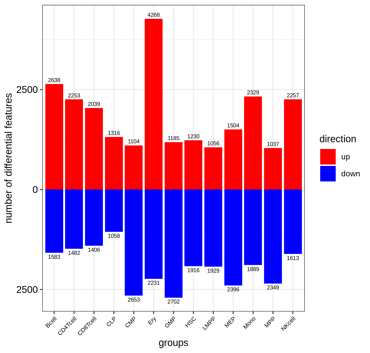
Bar plot of significantly differentially expressed gene counts split by directionality
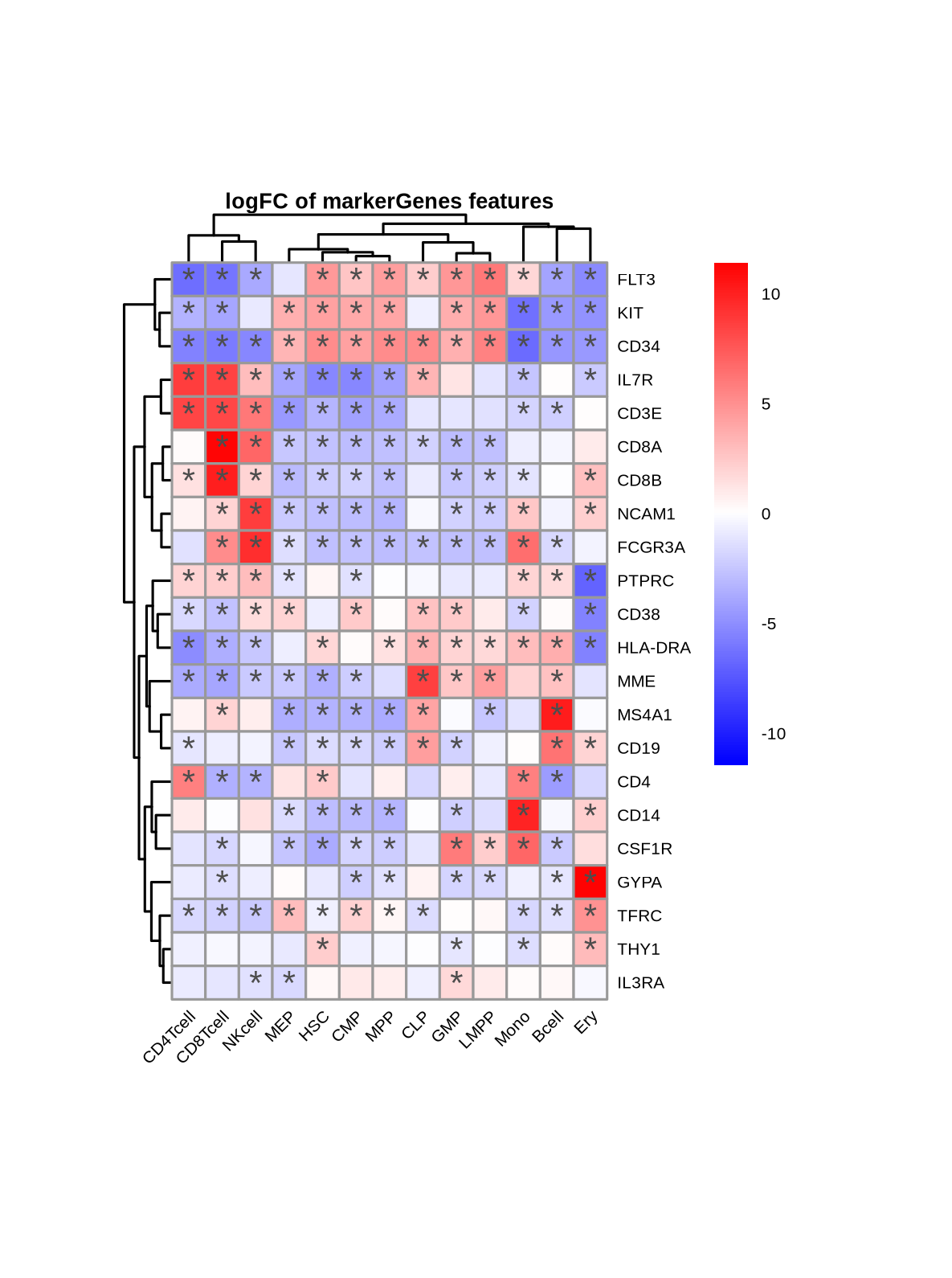
Heatmap of marker genes' DEA statistics across cell types (asterisks indicate statistical significance)
Note
Checkpoint: The directory results/CorcesRNA/dea_limma/normCQN_OvA_cell_type/feature_lists/ contains 13 files (e.g., Mono_featureScores_annot.csv), one for each comparison/cell type, listing all genes with their associated statistics score for downstream enrichment analysis.
4.7 • Biological Interpretation with enrichment_analysis
Configuration: config/CorcesRNA/CorcesRNA_enrichment_analysis_config.yaml
Annotation: config/CorcesRNA/CorcesRNA_enrichment_analysis_annotation.csv
To characterize and understand the biological functions underlying our cell-type-specific gene signatures, we perform enrichment analysis. Using the ranked gene lists with statistics scores from the previous step, the enrichment_analysis module performs a pre-ranked Gene Set Enrichment Analysis (GSEA). We query the Azimuth and Reactome databases to confirm cell type specificity and find biological processes or pathways that are significantly enriched among the differential genes for each cell type.
The results are aggregated and visualized as a bubble-heatmap, showing the top enriched terms for each cell type comparison. This provides a high-level biological interpretation of what differentiates or unites cell types.
| Azimuth 2023 | Reactome |
|---|---|
 |
 |
| Azimuth 2023 | Reactome |
|---|---|
 |
 |
Note
Checkpoint: Summary plots and tables are available in results/CorcesRNA/enrichment_analysis/cell_types/. The enrichment results are biologically plausible and align with the known functions of hematopoietic cell types.
Custom script: workflow/scripts/crossprediction.py
Note
The Crossprediction Method for Inferring Biological Similarity: Our crossprediction approach is a machine learning technique designed to quantify the similarity between biological groups based on their high-dimensional molecular profiles. It employs a Leave-One-Group-Out (LOGO) cross-validation strategy where a multi-class classifier (e.g., logistic regression) is trained on all groups except one, and then used to predict the class probabilities of the withheld group. The resulting prediction probabilities form a similarity matrix, where a high probability of misclassification between two groups indicates a high degree of similarity.
This method was first introduced by Farlik, Halbritter, et al. to computationally reconstruct the human hematopoietic lineage from DNA methylation profiles. It was later adapted by Traxler, Reichl, et al. to infer functional relationships between gene knockouts from scCRISPR-seq perturbation signatures, successfully validated by identifying members of known protein complexes.
Finally, to demonstrate the power of adding custom code to a modular workflow, we perform machine learning-based lineage reconstruction. We use a custom Python script (crossprediction.py) that trains a multinomial logistic regression classifier with elastic-net regularization for each cell type on the normalized and integrated highly variable feature dataset normCQN_integrated_HVF.
The script employs a Leave-One-Group-Out (LOGO) cross-prediction strategy to identify similarities between groups: to predict relationships for one cell type, it is held out, and a model is trained on all other cell types. The prediction probabilities of the held-out samples are aggregated into a similarity matrix. This (adjacency) matrix, when visualized as a graph, computationally reconstructs the human hematopoietic lineage, closely matching the known biological hierarchy.
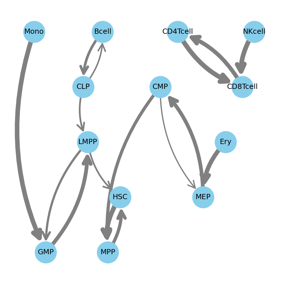
Crossprediction graph reconstruction of human hematopoietic lineage by similarity
We additionally leveraged the interpretability of logistic regression to identify the top five most positive predictive features (here genes) for every class (here cell type).
| Bcell | CD4Tcell | CD8Tcell | CLP | CMP | Ery | GMP | HSC | LMPP | MEP | MPP | Mono | NKcell |
|---|---|---|---|---|---|---|---|---|---|---|---|---|
| COL19A1 | CD4 | CD8A | EBF1 | CLC | PAQR9 | LILRB4 | ABCA13 | PRSS2 | HBB | HBB | VCAN | SH2D1B |
| FCRLA | TSHZ2 | LINC02446 | LINC01013 | MS4A2 | HBA2 | MPO | DLK1 | SPON1 | PKLR | LTBP1 | FCN1 | TRDJ1 |
| IGKC | ANKRD55 | CD8B | ARPP21 | EPX | GYPA | MPEG1 | RLIMP1 | DNTT | UBXN10 | CNRIP1 | S100A8 | AC093151.5 |
| TCL1A | F5 | AC022075.1 | RAG1 | IL5RA | TRIM10 | B3GNT7 | TCEAL2 | OPALIN | PLEKHG1 | FCER1A | S100A12 | GZMB |
| CNTNAP2 | CD40LG | ROBO1 | VPREB3 | PRG2 | IFIT1B | CCR2 | HLF | CCR7 | TGM2 | ITGB3 | SERPINA1 | DGKK |
Note
Checkpoint: The adjacency matrix is saved to results/CorcesRNA/special_analyses/crossprediction/adjacency_matrix.csv. When visualized, the resulting graph largely reflects the hierarchy of the human hematopoietic lineage.
Important
Explore the full interactive report:
This wiki page highlights key findings, but many more results are available for exploration. For a deeper dive, please see the complete interactive Snakemake report, where all outputs specific to this recipe are prefixed with CorcesRNA_*.
Even with a robust workflow, several issues can arise. Awareness of these potential problems can save significant time and prevent incorrect conclusions.
-
Poor Data Quality: As seen with sample
SRR2753109poor quality sample are not uncommon in biology. Low-quality reads can severely impact results. Always closely investigate QC results and remove outlier samples before proceeding with downstream analysis. - Resource Management: This analysis requires significant computational resources (~600GB disk space, ~3 hours on an HPC). Ensure adequate resources are available before starting. Running out of disk space mid-workflow can lead to downstream problems.
- Incorrect Normalization or Model: Choosing the wrong normalization method or model can fail to remove technical artifacts or worse, remove real biological signal. The confounding factor analysis is a critical diagnostic for choosing an appropriate method like CQN and inform the modeling approach.
- Limitation of ML interpretation: The computational lineage reconstruction demonstrates how easy it is to build your custom analyses on top of a modular workflow, but its simple interpretability approach has limitations. We identify genes that are positive predictors but will miss genes whose importance lies in being absent or down-regulated.
Note
Checkpoint: Before starting a new analysis, verify data quality, resource availability, and critically question the rationale of your analysis choices.
This section provides answers to common questions.
-
Why was Conditional Quantile Normalization (CQN) used? Our confounding factor analysis showed a significant association between gene expression and GC content. CQN is specifically designed to correct for such feature-level biases, in addition to library size, providing a more accurate representation of biological variation.
-
What is the purpose of the One-vs-All (OvA) differential expression analysis? The OvA strategy is ideal for finding a signature for each group in a multi-class experiment. By comparing each cell type to the average of all others, we identify genes that make that cell type distinct within the context of the entire system.
-
Why was the
donorvariable included in thelimmamodel? The data comes from multiple human donors, which can introduce biological and technical variability (a "batch effect"). Includingdonorin the model (~ 0 + cell_type + donor) allowslimmato estimate and account for this variability, increasing the statistical power to detect differences between cell types.
Important
Feedback, questions, or comments are very welcome, you can reach me via LinkedIn.