Single Particle In Uniform Magnetic Field - epicf/ef GitHub Wiki

In this example, we compare an exact analytical trajectory of a charged particle moving in a uniform magnetic field with results of a numerical simulation.

# To run the example:
cd your-ef-dir; cd examples/single_particle_in_magnetic_field; sh run_example.sh

A charged particle moves in uniform magnetic field in circular trajectory. An exact expressions for the trajectory can be obtained by solving Newton's equation:

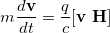
We chose z-axis to be directed along the magnetic field. Then the previous expression becomes:

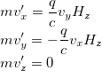
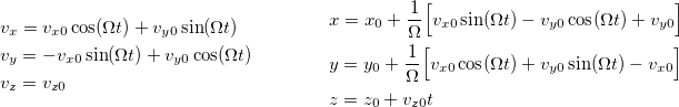
Performing integration over time (see Single Particle in Uniform Magnetic Field SymPy notebook), it is possible to obtain particle's law of motion:

The parameters of the circular motion - cyclotron frequency \Omega and Larmor radius r - are

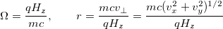
Let's perform some estimates. Suppose there is an electron (q = 4.8e-10 [cgs], m = 9.1e-28 [g]) moving in the 1000 [Gs] = 1 * 10^-1 [T] magnetic field. It's speed along the field (z-axis) corresponds to 1 keV energy, and it's speed in perpendicular plane corresponds to energy 100 eV (initially distributed evenly between x- and y-components). It's cyclotron frequency and Larmor radius are Omega = 1.633e+10 [1/s], r = 3.502e-02 [cm] ~ 0.035 [mm]. Gyration period equals to 3.848e-10 [s] and distance in the direction of the field covered during single revolution is 6.959e-01 [cm] ~ 7 [mm]

Now, to check this, in config file we define a source which generates a single particle at startup. Config is mostly similar to 'Singe Particle in Free Space' example, except this time we need nonzero magnetic field:

[External_magnetic_field_uniform.mgn_uni]
magnetic_field_x = 0.0
magnetic_field_y = 0.0
magnetic_field_z = 1000
speed_of_light = 3.0e10

Total simulation time has been adjusted to approximately 10 full gyration cycles (more precisely, 3.0e-9/3.848e-10 = 7.8 revolutions ).

[Time grid]
total_time = 3.0e-9 
time_step_size = 3.0e-12
time_save_step = 3.0e-12

Processing of simulation results is also mostly similar to the previous example. The law of motion is more complicated this time, and to define it we need not only particle mass and initial position and momentum, but also it's charge and magnitude of the magnetic field. All of this can be extracted from the relevant sections of the output *.h5 files. (see functions eval_an_trajectory_at_num_time_points, velocities and coords at plot.py)

Trajectory plots:

Apart from the trajectory, kinetic energy is also plotted. In theory, particle should not gain or loss any energy by interacting with magnetic field. However, due to numerical errors, this might not be the case in simulations. In this case, the energy is conserved.

Long Simulation Time
Boris integration scheme is notable for energy conservation even for long simulation times.

Time Step Larger Than Gyration Period
In practice it is necessary to keep in mind that time step should not exceed gyration period. Otherwise, this will lead to erroneous results.