Ribbon Beam Contour - epicf/ef GitHub Wiki

In this example we consider an evolution of a beam with rectangular cross section propagating in free space. Such beams are sometimes called ribbon beams.

# To run the example:
cd your-ef-dir; cd examples/ribbon_beam_contour; sh run_example.sh

Suppose there is a beam with rectangular cross section in the x-y plane, propagating along the z-axis. It's "height" (dimension along the y-axis) is much greater than it's "width" (dimension along the x-axis).

Due to particle-particle interaction, the beam widens as it propagates forward. If we consider an electron located on the x-axis edge of the beam, under certain approximations it is possible to obtain it's law of motion and the trajectory. For example, in the x-z plane it's trajectory is given by the following expression (in SI units):

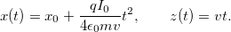
where I_0 is linear current density of the beam along the y-axis (i.e. full beam current I divided by beam "height"), \epsilon_0 is vacuum permittivity, v is speed along the z-axis, and x_0 and z_0 specify it's initial position.

A complete derivation of these relations can be found in a supplementary notebook; here we'll only state the employed approximations. First, for sufficiently "high" beam (large size along the y-axis) it is possible to assume that E_y = 0 for an electron in the middle of the beam. Second, if the beam has been propagating long enough time, so that it has acquired sufficient length, it is possible to approximate E_z = 0 at the points away from the front and the origin of the beam. Another assumption is that the charge density rho varies along the beam length (z-axis direction), but for a fixed z remains constant along the beam width (x-axis direction).

To compare the analytical model with the numerical simulation, it is possible to perform a numerical simulation of a beam propagating in free space and plot particles coordinates on the x-z plane.

todo: check config parameters and discuss estimates. Full simulation time is set to 3.0e-9 [s]. Source current is I = 0.01 [A] Total simulation time is 5 [ns], time step is 5 * 10^−12 [s]. Beam current is 0.008 [A], particles’ speed corresponds to 1 [keV] energy. 500 new macroparticles are added each time step.

After the simulation, X-Z coordinates of the particles are plotted.

Nonzero beam convergence angle

For nonzero initial beam convergence angle, trajectory of the electron on the x-axis edge of the beam is given by the following expression:

where is half thickness of beam in X direction, is beam convergence angle; I is linear current density of beam, U is accelerating voltage, which determines initial velocity of the particles, is charge/mass ratio , is vacuum permittivity.