04a 04 Merging Ordered and Time Series Data - ellen567/Data-Science-Notebook GitHub Wiki
Using merge_ordered()
- ordered data/time series
- Filling in missing values
- calling :
pd.merge_ordered(df1, df2) - forward fill: fills missing with previous value
fill_method='ffill'
merge_ordered() caution, multiple columns
- When using
merge_ordered()to merge on multiple columns, the order is important when you combine it with the forward fill feature. The function sorts the merge on columns in the order provided
date -> country
# Merge gdp and pop on country and date with fill
date_ctry = pd.merge_ordered(gdp, pop, on=['country','date'], fill_method='ffill')
output
         date country          gdp  series_code_x         pop series_code_y
0  2015-01-01   China  16700619.84  NYGDPMKTPSAKN  1371220000   SP.POP.TOTL
1  2015-01-01      US   4319400.00  NYGDPMKTPSAKN   320742673   SP.POP.TOTL
2  2015-04-01   China  16993555.30  NYGDPMKTPSAKN   320742673   SP.POP.TOTL
3  2015-04-01      US   4351400.00  NYGDPMKTPSAKN   320742673   SP.POP.TOTL
4  2015-07-01   China  17276271.67  NYGDPMKTPSAKN   320742673   SP.POP.TOTL
country -> date
# Merge gdp and pop on country and date with fill
date_ctry = pd.merge_ordered(gdp, pop, on=['country','date'], fill_method='ffill')
output
         date country          gdp  series_code_x         pop series_code_y
0  2015-01-01   China  16700619.84  NYGDPMKTPSAKN  1371220000   SP.POP.TOTL
1  2015-04-01   China  16993555.30  NYGDPMKTPSAKN  1371220000   SP.POP.TOTL
2  2015-07-01   China  17276271.67  NYGDPMKTPSAKN  1371220000   SP.POP.TOTL
3  2015-09-01   China  17547024.54  NYGDPMKTPSAKN  1371220000   SP.POP.TOTL
4  2016-01-01   China  17820789.83  NYGDPMKTPSAKN  1378665000   SP.POP.TOTL
Using merge_asof()
- Similar to a
merge_ordered()left_join- similar features as
merge_ordered()
- similar features as
- Match on the nearest key column and not exact matches.
- Merge 'on' colomns must be sorted.
direction='forward',direction='nearest'
Selecting data with .query()
.query('some selection statement')stocks.query('nike >= 90')stocks.query('nike > 90 and disney < 140')stocks_long.query('stock=="disney" or (stock=="nike" and close<90)')
Reshaping data with .melt()
- The melt method allow us to unpivot our dataset to long format
In [2]: ten_yr.head()
Out[2]:
  metric  2007-02-01  2007-03-01  2007-04-01  2007-05-01  ...  2009-08-01  2009-09-01  2009-10-01  2009-11-01  2009-12-01
0   open    0.033491   -0.060449    0.025426   -0.004312  ...   -0.006687   -0.046564   -0.032068    0.034347   -0.050544
1   high   -0.007338   -0.040657    0.022046    0.030576  ...    0.031864   -0.090324    0.012447   -0.004191    0.099327
2    low   -0.016147   -0.007984    0.031075   -0.002168  ...    0.039510   -0.035946   -0.050733    0.030264    0.007188
3  close   -0.057190    0.021538   -0.003873    0.056156  ...   -0.028563   -0.027639    0.025703   -0.056309    0.200562

[4 rows x 36 columns]
# Use melt on ten_yr, unpivot everything besides the metric column
bond_perc = ten_yr.melt(id_vars='metric', var_name='date', value_name='close')
In [3]: bond_perc.head()
Out[3]:
metric date close
0 open 2007-02-01 0.033491
1 high 2007-02-01 -0.007338
2 low 2007-02-01 -0.016147
3 close 2007-02-01 -0.057190
4 open 2007-03-01 -0.060449
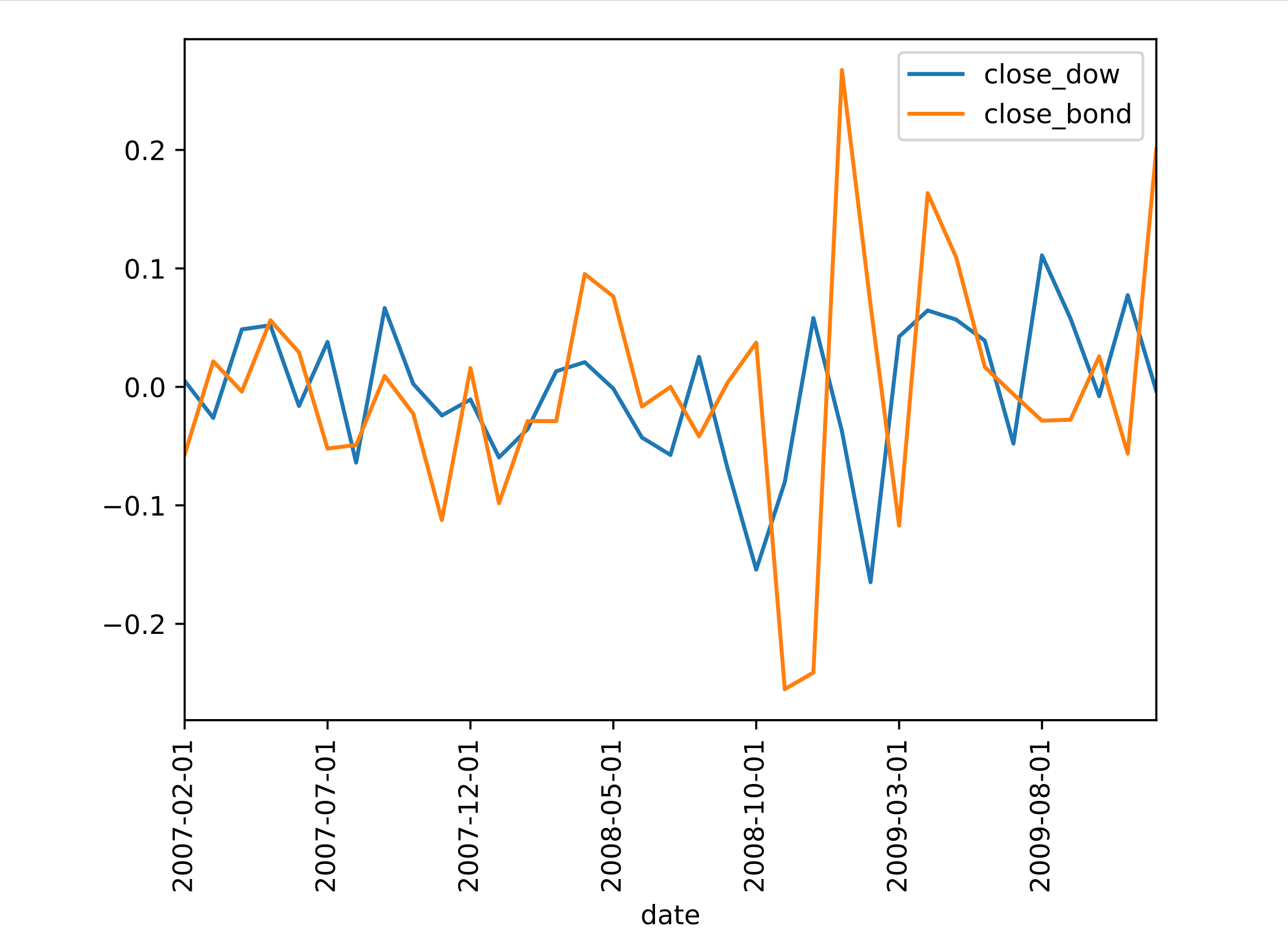
In [4]: dji.head()
Out[4]:
date close
0 2007-02-01 0.005094
1 2007-03-01 -0.026139
2 2007-04-01 0.048525
3 2007-05-01 0.052007
4 2007-06-01 -0.016070
# Use query on bond_perc to select only the rows where metric=close
bond_perc_close = bond_perc.query('metric=="close"')

# Merge (ordered) dji and bond_perc_close on date with an inner join
dow_bond = pd.merge_ordered(dji, bond_perc_close, on='date', how='inner',suffixes=['_dow','_bond'])
In [5]: dow_bond.head()
Out[5]:
         date  close_dow metric  close_bond
0  2007-02-01   0.005094  close   -0.057190
1  2007-03-01  -0.026139  close    0.021538
2  2007-04-01   0.048525  close   -0.003873
3  2007-05-01   0.052007  close    0.056156
4  2007-06-01  -0.016070  close    0.029243
# Plot only the close_dow and close_bond columns
dow_bond.plot(y=['close_dow','close_bond'], x='date', rot=90)
plt.show()