8. Modeling: Linear Regression - eliasmelul/CrimeInvestigation GitHub Wiki
Numerous models and transformations were considered and constructed in addition to the models discussed in this section. However, we concluded that it wasn’t appropriate to make any transformations due to the nature and relationships of the datasets being used.
Intuitive Linear Regression Model
A linear regression model was conducted, in which the estimation model can be illustrated as:
Frequency = Intercept + Avg_Temp + DoW + Events
where Avg_Temp is represented with integers, and DoW and Events are binary indicators of each day of the week and the events of precipitation, respectively. Based on our data exploration, we believe that that the best predictors for crime rate are (1) the average temperature, (2) the day of the week, and (3) the event – Rain, None, Snow, or Both. Average Dew Point was excluded due to the extremely high correlation with average temperature. The model is summarized in the following table:
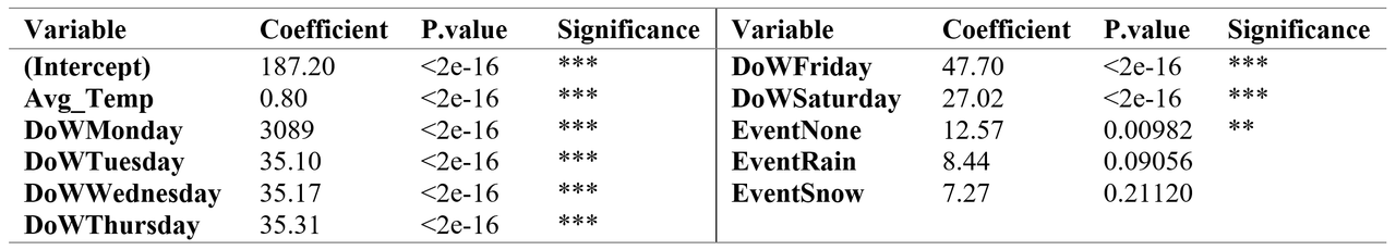
The intuitive model of Figure 8 delivers an adjusted R-squared of 0.3573 and AIC of 9682.215. All variables are significant at 99.9% except for EventRain and EventSnow. According to this model, with everything else constant, weekdays tend to have a higher average for the number of crimes per day with Sunday being the day with the least average amount of crimes by 27 crimes. Furthermore, crimes tend to increase by 12 crimes per day if doesn’t rain and snow and increase by 0.8 crimes for every increase in the average temperature (F). Since our range for average temperature is 86 Fahrenheit, with a minimum of 2 Fahrenheit, the increase amount of the count of the daily crimes can be up to 69 daily crimes within the set of average temperatures recorded.
Backward Selection Model
A backward selection model was conducted, in which the estimation model can be illustrated as:
Frequency = Avg_Dew_Point + Avg_Humidity + Avg_Visibility + DoW
where Avg_Dew_Point, Avg_Humidity, and Avg_Visibility are represented with integers, and DoW is a binary factorized variable for each day of the week. A summary of the model is described below:
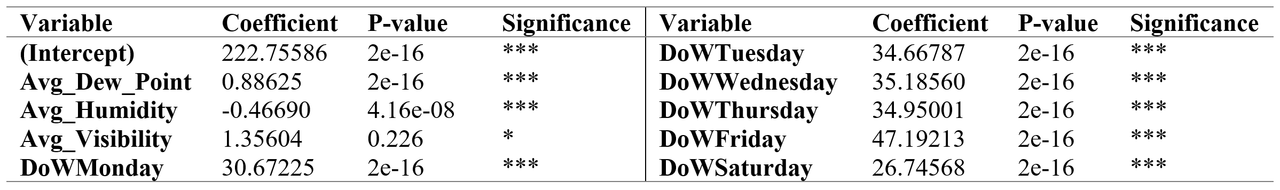
From running a backward selection model on our dataset, we found the weekdays to have a higher average crime rate than the weekends, with Sunday at the lowest and Saturday as the second lowest. We see that the average dew point and humidity are also highly statistically significant in predicting the crime rates in this model. With the daily crime rate as the independent variable, the model gets an adjusted R-squared value of 0.3663 and an AIC of 9666.663. With a resembling interpretation of the coefficients as the Intuitive model, we also have a level-log relationship between the average humidity (represented as a percentage) and the crime rate. This relationship can be interpreted as, with all other factors unchanged, per every percent increment of the average humidity, the crime rate decreases by roughly half percent.
Forwards and Stepwise Selection Model
Both selection models had the same outcome.
A forward and stepwise selection model was conducted, in which the estimation model can be illustrated as:
Frequency = Avg_Temp + Avg_Visibility + DoW
where Avg_Temp and Avg_Visibility are represented with integers, and DoW is a binary indicator of each day of the week. A summary of the model is described below:
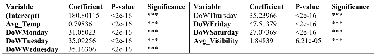
The forward selection model and stepwise selection model end up yielding the exact same model. As figure 10 shows, all the variables in the model are highly significant to the model. When looking at “day of the week”, the model shows that, compared to Sundays, weekdays have a higher average crime rate holding all other variables constant. With the daily crime rate as the independent variable, we get the average temperature, the average visibility, and the day of the week with an adjusted R-squared value of 0.3616 and an AIC of 9673.246. When comparing the R-squared value and the AIC between the backward selection model and the forward and stepwise selection model, we can see that the values are very similar to each other.
Assumption Check - Intuitive Model
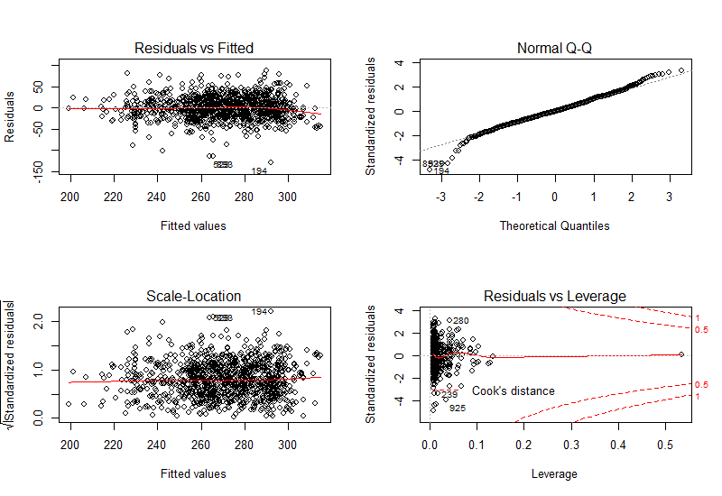 Figure 16. Residual vs. Fitter (upper left), Normal Quantile-Quantile (upper right), Scale vs. Location (bottom left), Residuals vs. Leverage (upper right)
- From the residual versus fitted graph, we can observe that the number of data points above and below the red line are roughly the same, demonstrating that the mean of the residuals is 0. Furthermore, we observe a quasi-constant distribution of data, indicating linearity of the model.
- From the normal quantile to quantile plot, we can see that the data passes the “fat pencil test” indicating normality of data except for the lower tail of data.
- The residual versus leverage plot shows that there is only one high-leverage observation with a cook’s distance (distance from centroid) below 0.5, hence the model doesn’t seem to be significantly influenced by outliers.
Discussion and Evaluation
A correlation between weather and crime rate in Boston has been observed from the years 2015 to 2018. The frequency of crimes tends to move drastically with Boston’s seasonal changes, where there is an overall higher count during the summer following a lower count in the winter. According to the intuitive linear regression model, a unit increase in the temperature (degree) results in an increase in the daily crime rate by a statistically significant value of approximately 187 records. This could possibly be explained by the inclination of people to be more active during warmer, endurable temperatures than during the winter of Boston, which is commonly known to be very cold. Furthermore, it has been observed that the crime rate is significantly higher during the weekdays than during the weekend. As depicted in both the forward and backward selection models, the crime rate recorded between the years 2015 and 2018 gradually increases from Monday to Friday and declines on Saturday and even further on Sunday, all of which have been established as statistically significant results.
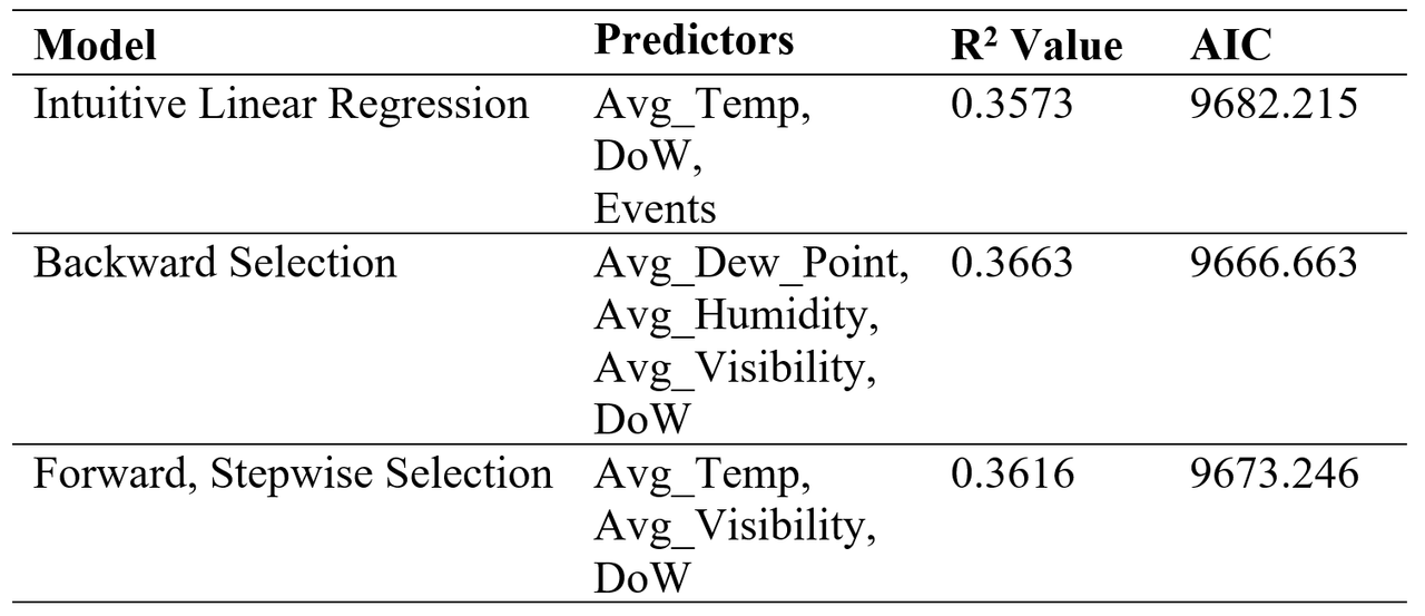
From the table above, we can see that the backward selection model has the largest R-square value and the smallest AIC value compared to the other two models. Accordingly, the backward selection model interprets the crime frequency relatively better but is not as intuitive as the intuitive linear regression model. We also notice that all the models provide a similar story with most important variables relating to the average temperature and day of week, with the goodness of fit coefficients of the three models being extremely close. Therefore, we choose to keep the Intuitive Linear Regression Model for crime rate prediction.
It is important to address that the results obtained from this study do not assure complete knowledge and prediction of the crime tendencies within specific locations of Boston during each season. This study only observes the past occurrences of crime in order to help raise awareness of possible criminal activity in certain areas of Boston during a certain period of the year. In addition, it is likely that not all crimes have been reported to the police department for multiple reasons such as fear to report. Therefore, a dataset covering more years of records on crime and on temperature would increase the accuracy of our results.