This page contains technical information intended for developers.

I will first explain the relevant concepts in the context of three-phase, then I will explain how the concepts can be extended to an arbitrary number of phases.

Position encoding for three-phase

The position is a concept for describing where you feel the sensation. By sending successive pulses with different position values, a moving sensation can be generated.

Position and intensity are independent.

For three-phase, the position has 2 degrees of freedom, alpha and beta. A diagram is show below, the green dot indicates the position.

TODO: annotate with direction of alpha/beta axis. Positive alpha points to the Neutral, positive beta points to the left at a 90° angle with alpha.

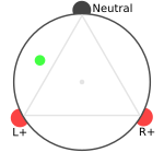
• A position on the center equally stimulates all 3 electrodes.
• A position on the neutral maximally stimulates the neutral electrode (1) and minimally stimulates left/right (0.5 each). And vice-verse for left and right.
• A position directly opposite the neutral only stimulates left and right. And vice-verse for left and right.

Reference code for translating position to electrode intensity (threephase only):

from numpy import sqrt, dot, sin, cos, arctan2
from numpy.linalg import norm

v1 = [1, 0]                 # neutral
v2 = [-0.5, sqrt(3) / 2]    # left
v3 = [-0.5, -sqrt(3) / 2]   # right
# v1 + v2 + v3 == 0

position = (0.8, 0.1)       # your (alpha, beta) here
r = norm(position)
assert(r <= 1)

# three-phase only: the angle is halved
theta = arctan2(position[1], position[0])
position = (cos(theta/2) * r, sin(theta/2) * r)

neutral_intensity = (1 - r) + abs(dot(v1, position))
left_intensity    = (1 - r) + abs(dot(v2, position))
right_intensity   = (1 - r) + abs(dot(v3, position))

For stereostim waveforms, the intensity is the uncalibrated waveform amplitude.

Honeycomb diagram in three-phase

The honeycomb diagram is a tool for visualizing the waveforms of individual pulses, suitable both for analog and pulse-based devices.

The axis setup is slightly different than for position encoding, also utilizing the variables alpha and beta. These should not be confused with the position alpha and beta.

The unit of choice can be voltage, current, or charge. Charge being the most logical choice.

There is a direct translation from the position to the 6 bounds of the diagram (code in the previous section). Bounds are always hexagonal with all angles at 120°.

For pulse-based devices such as the NeoDK with 'digital' signal generation, signals move parallel to any of the bounds.

To translate between the honeycomb diagram and electrode waveform, use the alpha-beta transform.

Calibration in three-phase

Calibration is needed to correct for these things:

• Asymmetries in traditional stereostim boxes.
• Different electrode shape, size, material and impedance.
• Different nerve sensitivity.

These goals can be reached with two simple transformations.

Neutral/left/right calibration

For this calibration there are two variables, neutral_calibration and left_calibration, unit Decibel.

neutral_calibration is defined as a scale of the honeycomb in the neutral axis, this can be used to increase or decrease neutral electrode power relative to the left or right electrode.

left_calibration is defined as a scale of the honeycomb at an axis 45° degrees from neutral. This has the net effect of increasing the left electrode power relative to left, in a way that is as orthogonal as possible to neutral_calibration.

Reference code (analog devices):

from stim_math.threephase import ab_transform, ab_transform_inv
import numpy as np

def scale_in_arbitrary_direction(a, b, scale):
    # formula from:
    # https://computergraphics.stackexchange.com/questions/5586/what-does-it-mean-to-scale-in-an-arbitrary-direction
    s = (scale - 1)
    return np.array([[1 + s * a**2, s * a * b],
                     [s * a * b, 1 + s * b**2]])

def generate_transform_in_ab(neutral, left):    # calibration values
    if (neutral, left) == (0, 0):
        return np.eye(2)
    theta = np.arctan2(left, neutral) / 2
    ratio = 10 ** (np.linalg.norm((neutral, left)) / 10)
    return scale_in_arbitrary_direction(np.sin(-theta), np.cos(theta), 1/ratio)


calibration_neutral = 1     # your values here
calibration_left = -0.5      # your values here

transform = generate_transform_in_ab(calibration_neutral, calibration_left)
transform = ab_transform[:3, :2] @ transform @ ab_transform_inv[:2, :3]

# perform calibration on electrode signals
(signal_neutral, signal_left, signal_right) = transform @ (signal_neutral, signal_left, signal_right)

TODO: figure out for pulse-based devices.

Center calibration

Even with neutral and left calibration, positions in the center still tend to feel stronger, center calibration corrects for this by multiplying the signal intensity with some value.

Values around -0.5 to -0.7 are usually good.

Reference code:

def get_scale(center_calibration, alpha, beta):  # position coordinates
    ratio = 10 ** (center_calibration / 10)
    norm = np.norm(alpha, beta).clip(min=None, max=1)

    if ratio <= 1:
        edge = 1
        center = ratio
    else:
        edge = 1/ratio
        center = 1

    return center + norm * (edge - center)

Extensions

The position encoding always generates rotationally symmetric honeycombs around the origin. However, for balanced biphasic pulses it is only required that the honeycomb contains the origin (unit = charge). Pulses that mimic anode-first or cathode-first sensations can thus be generated by offsetting the honeycomb from the origin.

Position encoding for many-phase

With 3 electrodes, the position is a point in a 2D circle. With 4 electrodes, it is a point in a 3D ball. With 5 electrodes, a point in 4D ball.

Basis vectors for 3 electrode configs:

v1 = [1, 0]
v2 = [-0.5, sqrt(3) / 2]
v3 = [-0.5, -sqrt(3) / 2]
v1 + v2 + v3 == 0

Basis vectors for 4 electrode configs:

COEF_1 = 1
COEF_2 = sqrt(8) / 3        # sqrt(1 - coef_1**2/3)
COEF_3 = sqrt(2) / sqrt(3)  # sqrt(1 - coef_1**2/3 - coef_2**2/2)

v1 = [COEF_1, 0, 0]
v2 = [-COEF_1 / 3, COEF_2, 0]
v3 = [-COEF_1 / 3, -COEF_2 / 2, COEF_3]
v4 = [-COEF_1 / 3, -COEF_2 / 2, -COEF_3]
v1 + v2 + v3 + v4 == 0

Basis vectors for 5 electrode configs:

COEF_1 = 1
COEF_2 = sqrt(15) / 4       # sqrt(1 - coef_1**2/4)
COEF_3 = sqrt(5) / sqrt(6)  # sqrt(1 - coef_1**2/4 - coef_2**2/3)
COEF_4 = sqrt(5) / sqrt(8)  # sqrt(1 - coef_1**2/4 - coef_2**2/3 - coef_3**2/2)

v1 = [COEF_1, 0, 0, 0]
v2 = [-COEF_1 / 4, COEF_2, 0, 0]
v3 = [-COEF_1 / 4, -COEF_2 / 3, COEF_3, 0]
v4 = [-COEF_1 / 4, -COEF_2 / 3, -COEF_3 / 2, COEF_4]
v5 = [-COEF_1 / 4, -COEF_2 / 3, -COEF_3 / 2, -COEF_4]
v1 + v2 + v3 + v4 + v5 == 0

Code is the same as the three-phase code given earlier, only the step to halve the angle is skipped if there are more than 3 electrodes.

The reason is that the full phase diagram contains 2 points with the same sensation. For three-phase, we map half the circle to a full circle and display that to the user. This gets rid of the duplicates. But no such mapping exists in 3D or higher.

Honeycomb diagram for many-phase

For 4-phase the 2D honeycomb is replaced by a 3D regular octahedron. And for 5-phase, a 4D object enclosed within 5 sets of parallel surface.

Visualization becomes more complicated, but the basic concept is still useful for signal generation.

Calibration for many-phase

An intuitive approach is most likely impossible.

This means calibration in N-phase will involve N variables instead of N-1. This almost certainly requires a current-controlled device.