Mission Analysis - cubesat-project/CubeSat GitHub Wiki

Description of Mission Analysis

Satellite orbital lifecycle assessment serves to inform the satellite mission preparation, operational cycle, and post-operational analysis. Determining orbit parameters in Low Earth Orbit (LEO) and examining orbital perturbation factors for the decay of the satellite orbit ensures a greater accuracy of the predicted orbit and lifespan of the satellite. The orbit analysis and determination ensures the accurate tracking of the satellite, confirmed by observational data upon deployment.

Background

Satellite orbit factors of consideration:

Gravitational effect between the satellite orbiting body and the primary body
Orbit perturbations:
Gravitation effects of the non-uniform mass distribution of the Earth
Atmospheric air drag in LEO
Solar radiation pressure emitted as delayed infrared radiation (IR)
Solar radiation emitted by albedo reflected from the Earth

Keplerian Orbital Parameters

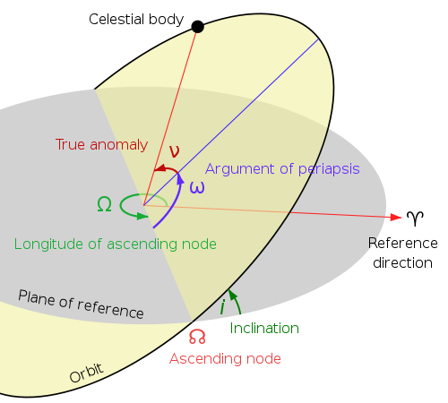
Describes the size and shape of orbit:

Semi-major axis (a)
Eccentricity (e)

Describes the orientation of the orbit in space:

Inclination (i)
Right ascension of the ascending node (Ω)
Argument of perigee (ω)

Describes the location of satellite within the orbit

True anomaly (v)

Computational Methodologies

Encke’s formulation: Uses osculating orbit to integrate the difference between two-body acceleration and perturbed acceleration.
Cowell’s formulation: Uses perturbing acceleration factors for numerical integration using the equations of motion.

Runge-Batta technique for the single-step method: Evaluates the system of equations at several intermediate steps similarly to fourth-order Taylor series.
Adams-Bashforth-Moulton and Shampine-Gordon fourth-order method: Multi-step predictor-corrector methods.

General Perturbation Techniques: Uses analytical approximations of the satellite motion over a time interval with initial condition data.

Lagrange Variation of Parameters (VOP): Uses the generalized Lagrange planetary equations of motion for non-linear integral systems and changing orbital parameters in the two-body equations.
Gaussian Variation of Parameters (VOP): Shows the rate of change of the non-conservative forces expressed directly by the perturbing acceleration.

Systems Tool Kit (STK)

What is STK? STK is a physics-based software used to visualize the system’s model and evaluate its contextual performance. This package is offered by Analytics Graphics, Inc. (AGI). The software is not MacOs compatible and also no longer supported on Windows 7,8 and server 2008 R2. For any kind of analysis, users are required to first create or open what is known as a scenario upon starting STK. A scenario is an STK file where all the design and analysis takes a place. Based on the time period provided for a scenario, STK GUI will be displayed. Three main parts of the GUI are the following: a 3d graphics window to visualize the planet under analysis, a 2d graphics window with the same purpose and a timeline view window. From there, the user can add objects such as satellites, aircrafts and targets, and study their interactions. Each object has a set of properties (e.g. model for satellites) that can be further customized to fit the user’s purpose.

STK-Level 1

There are 3 levels of Systems Tool Kit certification, level 1 covers the fundamental skills necessary to use the free version of STK. This includes building basic scenarios, generating reports, and recording videos. Training at this level is necessary for orbit analysis for Ukpik-1.

Tutorials included in L1 training:

Create a New Scenario
Insert STK Objects; ground sites, vehicles, and sensors
Modify STK Objects; to customize object properties such as range constrains and orbits
Compute Access; to calculate object-to-object visibility
Create Reports & Graphs
Send Connect Commands; the connect module holds a library of string commands to read, understand, and build
Make a Movie; to depict complex concepts/relationships which would otherwise be difficult to visualize

Screenshot from STK Version 10, including the object browser, 2D graphics window, 3D graphics window, and timeline view.

STK-Level 2

Converting CAD Model for use in STK

Software used:Blender 2.83

Scale and Align

Import .stl model into Blender
select model, ctrl+A, select "scale" and set Scale X,Y,Z
Make sure you are in the "Layout" workspace at the top, select "Object" > "Set Origin" > "Geometry to Origin"
Set Rotation X to 90d to rotate CubeSat 90 degrees about x axis

Separating solar cells into their own objects in Blender

On the upper left corner, set the mode to "Edit Mode"
Click on "Face Select" next to the mode dropdown menu
Select all the solar panels on one face of the CubeSat
Press P or alternatively at the top click on "Mesh"> "Separate" > "Selection"
Repeat the process for the remaining 3 sides of the CubeSat
Now the objects should appear separately on the right, under "Scene Collection"
By double clicking on the object name in the list on the right, you can rename it

Add New Material for the CubSat body and solar cells

Select the body object (i.e. the object without any solar cells)
On the right, click on the "Materials Properties" icon and add a new material
Do the same for each solar panel object, but set the "Base Color" to something different

Attach the Child Solar Panels onto the Parent CubeSat Body

Select the child (solar panel) and then the parent (CubeSat body), the parent should be contoured in a lighter colour than the child, indicating that that is the active object
Right click > "Parent" > "Object"
You can now see on the right that the solar panel object appears as a sub-object of the CubeSat body object
Save as .blender file
Export as .gITF file (STK-compatible)

Creating the GMDF File

GMDF outlines the properties of your model (e.g. solar cell efficiency) and can be edited
to set up a GMDF file visit https://github.com/AnalyticalGraphicsInc/gmdf

Sun Angles and Sun Exposure

Orbital Lifetime

Ground Station Access

CSA Webinar Notes (Orbit-related)

Webinar 2-3

Webinars2-3 Summary

Webinar 15: Intro to B-dot Control Law for Attitude Control Subsystem (ACS)

Why do we need attitude control? To orient the satellite in the direction we want.
Once ejected from the ISS, Ukpik-1 will be tumbling, this needs to stop for antennas, sensors, trackers, and solar panels to be effective.

Detumbling is the process of reducing initial angular velocity to a point where the sensors aboard the satellite are of use again.

How to detumble using the design of your satellite:

Using 3 magnetorquers on mutually perpendicular axes, magnetorquers use Lorentz forces and work best at LEO (where Earth’s magnetic field is stronger).

To detumble, the magnetic moment should be in the negative direction.

Using a permanent magnet (for a constant magnetic moment).

Doesn’t require power, however, its strength cannot be controlled and the magnet cannot be turned off, so it will interfere with the magnetometer readings. To compensate for this a ‘bias’ could be added to the magnetometer reading that subtracts the readings from the permanent magnet.

We will also need a 3-axis magnetometer, which is equipped with sensors to read the local magnetic field direction and strength after the satellite has become stable.

IMPORTANT NOTE: Earth’s magnetic field is NOT uniform with geographic location, which is why we need a magnetometer.

B-dot Control Law for magnetorquers and magnetometers (note: these cannot be used simultaneously, because magnetorquers generate their own magnetic field).

All you need to use B-dot Control Law are regular readings of the magnetic field (a magnetometer). B-dot = the change in magnetic field strength over time, directly proportional to angular velocity (ex. If the magnetometer readings are changing rapidly, the satellite is spinning fast). The satellite should be able to detumble within 2-3 orbits of Earth (3-5 hours from launch).