Overview of Deep Learning Algorithms - clizarraga-UAD7/Workshops GitHub Wiki
(Image credit: CC Viterbi School of Engineering, University of Souther California)

From Wikipedia:
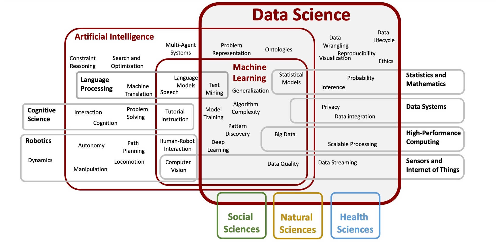
Deep learning is part of a broader family of machine learning methods based on artificial neural networks with representation learning. Learning can be supervised, semi-supervised or unsupervised.
Deep-learning architectures such as deep neural networks, deep belief networks, deep reinforcement learning, recurrent neural networks, convolutional neural networks and Transformers have been applied to fields including computer vision, speech recognition, natural language processing, machine translation, bioinformatics, drug design, medical image analysis, climate science, and board game programs, where they have produced results comparable to and in some cases surpassing human expert performance.
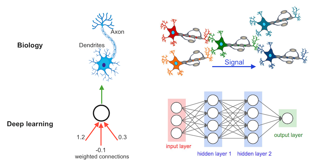
A biological neuron is the basic unit of the nervous system, transmitting information via electrical and chemical signals. It receives and processes signals through its dendrites and cell body, then sends outputs through its axon. This process facilitates critical interactions for thought, sensation, movement, and body function regulation.
An artificial neuron is a mathematical model that behaves like a biological neuron. It takes one or more inputs, each weighted by importance, sums them, and processes the sum through a nonlinear activation function. The output can then feed into other neurons. The weight adjustments based on network performance are the basis of learning in artificial neural networks.
When comparing biological neurons to artificial ones, the soma (cell body) is similar to the node, dendrites (signal receivers) correspond to the inputs, synapses (connections between neurons) are equivalent to weights or interconnections, and the axon (signal transmitter) parallels the output.
The evolution of neural networks, a captivating journey through AI progression, introduced sophisticated models for complex problems. Here are the key milestones and their contributions:
- The perceptron model
- The multilayer perceptron (MLP)
- Convolutional neural networks (CNNs)
- Sequential models
- Transformers
- Large language models (LLMs)
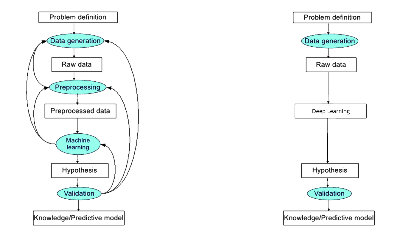
The process of training a model in Deep Learning is directly inputting the data into the model. The model will learn and perform the classification.

Image credit: Sebastian Raschka
At a basic level, a neural network is comprised of four main components: inputs, weights, a bias (or threshold or intercept), and an output. Similar to linear regression, the algebraic formula would look something like this:
The above equation for the prediction value
Example
Example: Whether or not you should order a pizza for dinner. This will be our predicted outcome, or
Let’s assume that there are three main factors that will influence your decision:
- If you will save time by ordering out (Yes: 1; No: 0)
- If you will lose weight by ordering a pizza (Yes: 1; No: 0)
- If you will save money (Yes: 1; No: 0)
Then, let’s assume the following, giving us the following inputs:
-
$x_1 = 1$ , since you’re not making dinner -
$x_2 = 0$ , since we’re getting ALL the toppings -
$x_3 = 1$ , since we’re only getting 2 slices
For simplicity purposes, our inputs will have a binary value of 0 or 1. This technically defines it as a perceptron as neural networks primarily leverage sigmoid neurons.
Next need to assign some weights to determine importance. Larger weights make a single input’s contribution to the output more significant compared to other inputs.
-
$w_1 = 5$ , since you value time -
$w_2 = 3$ , since you value staying in shape -
$w_3 = 2$ , since you've got money in the bank
Finally, we’ll also assume a threshold value of 5, which would translate to a bias value of –5.
Using the following activation function, we can now calculate the output (i.e., our decision to order pizza):
$$ {\rm output}: \ \ \ f(x) = 1 \ \ if \ \ \hat{y} \ge 0 \ \ \ else \ \ \ f(x) = 0 \ $$
In summary:
$$ \begin{eqnarray} \hat{y} & = & (5 * 1) + (3 * 0) + (2 * 1) - 5 \ & = & 5 + 0 + 2 – 5 \ & = & 2 \ \end{eqnarray} $$
Since
💻 Try this visual interactive neural network
Loss functions quantify the distance between the real and predicted values of the target. The loss will usually be a non-negative number where smaller values are better and perfect predictions incur a loss of 0. For regression problems, the most common loss function is squared error.

When we measure the loss as a sum of squares of the differences, we may end up with large quantities, especially when there are some outlier data. To measure the quality of a model on the entire dataset of
When training the model, we want to find the optimal parameters
Optimization algorithms train neural networks. These algorithms are also called optimizers. There are various types of optimizers; each type has its characteristics. The performance-optimizing algorithms depend on the processing speed, memory requirement, and computational accuracy. The process of optimization can either be one-dimensional or multidimensional.
The key technique for optimizing nearly any deep learning model consists of iteratively reducing the error by updating the parameters in a direction that incrementally lowers the loss function. This algorithm is called stochastic gradient descent.
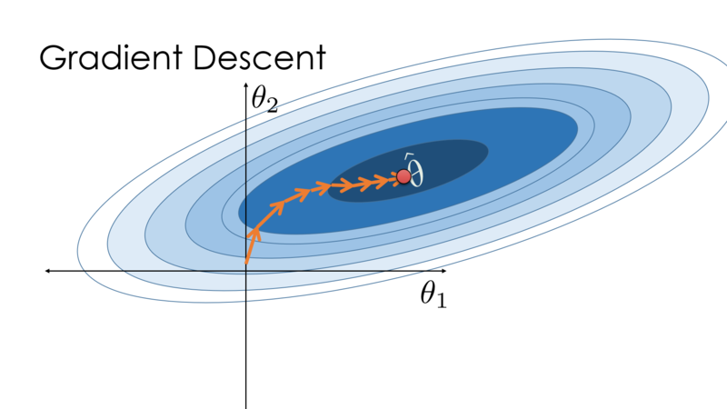
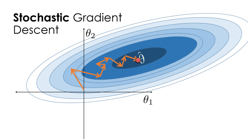
Image Credit: Cornell's University Computational Optimization Textbook
Gradient descent is typically the slowest training algorithm. The Levenberg-Marquardt algorithm may be the fastest one, but it typically takes a lot of memory. The quasi-Newton approach could be a reasonable compromise. The Levenberg-Marquardt algorithm might be the best choice if we have many neural networks to train. The quasi-Newton approach would fit well in the majority of the scenarios.

Image credit: Sebastian Raschka
The simplest deep networks are called multilayer perceptrons, and they consist of multiple layers of neurons each fully connected to those in the layer below (from which they receive input) and those above (which they, in turn, influence).
Let's exemplify with a neural network with L=3 layers.

Image credit: Sebastian Raschka
The above model with m=3 input variables (3 variables with
If
where
The prediction of the model is given by the output vector
In order to realize the potential of multilayer architectures, we need one more key ingredient: a nonlinear activation function
To build more general multilayer neural networks, we can continue stacking such hidden layers, e.g.,
There is no definitive guide for which activation function works best on specific problems. It’s a trial and error process where one should try a different set of functions and see which one works best on the problem at hand.
There are several options for selecting activation functions:
- Rectified Linear Unit (ReLU):

- The sigmoid function transforms its inputs, for which values lie in the domain R, to outputs that lie on the interval (0, 1):

- Like the sigmoid function, the tanh (hyperbolic tangent) function also squashes its inputs, transforming them into elements on the interval between -1 and 1:

The input
The architecture of the network entails determining its depth, width, and activation functions used on each layer. Depth is the number of hidden layers. Width is the number of units (nodes) on each hidden layer since we don’t control either the input layer or output layer dimensions.
Research has proven that deeper networks outperform networks with more hidden units. Therefore, it’s always better and won’t hurt to train a deeper network.
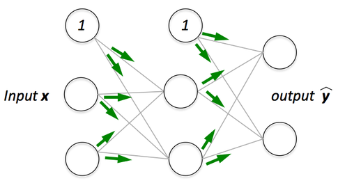
If we have a multi-layer neural network, we can picture forward propagation (passing the input signal through a network while multiplying it by the respective weights to compute an output) as follows:
And in backpropagation, we “simply” backpropagate the error (the “cost” that we compute by comparing the calculated output and the known, correct target output, which we then use to update the model parameters):
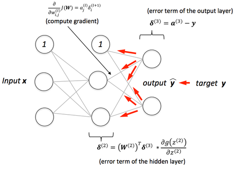
Images credit: Sebastian Raschka
Feedforward neural networks (FF or FFNN) and perceptrons (P)

A feedforward neural network is an artificial neural network wherein connections between the nodes do not form a cycle. As such, it is different from its descendant: recurrent neural networks. The feedforward neural network was the first and simplest type of artificial neural network devised.
Examples:
Radial Basis Function (RBF)

In the field of mathematical modeling, a radial basis function network is an artificial neural network that uses radial basis functions as activation functions. The output of the network is a linear combination of radial basis functions of the inputs and neuron parameters.
Recurrent neural networks (RNN)

A recurrent neural network is a class of artificial neural networks where connections between nodes can create a cycle, allowing output from some nodes to affect subsequent input to the same nodes. This allows it to exhibit temporal dynamic behavior.
Long / short-term memory (LSTM)

Long short-term memory is an artificial neural network used in the fields of artificial intelligence and deep learning. Unlike standard feedforward neural networks, LSTM has feedback connections. Such a recurrent neural network can process not only single data points but also entire sequences of data.
Gated recurrent units (GRU)

Gated recurrent units are a gating mechanism in recurrent neural networks, introduced in 2014 by Kyunghyun Cho et al. The GRU is like a long short-term memory with a forget gate, but has fewer parameters than LSTM, as it lacks an output gate.
Bidirectional recurrent neural networks, bidirectional long/short-term memory networks, and bidirectional gated recurrent units (BiRNN, BiLSTM, and BiGRU respectively)
Bidirectional recurrent neural networks, bidirectional long/short-term memory networks, and bidirectional gated recurrent units (BiRNN, BiLSTM, and BiGRU respectively)

Bidirectional recurrent neural networks connect two hidden layers of opposite directions to the same output. With this form of generative deep learning, the output layer can get information from past and future states simultaneously.
Autoencoders (AE)

An autoencoder is a type of artificial neural network used to learn efficient codings of unlabeled data. The encoding is validated and refined by attempting to regenerate the input from the encoding. The autoencoder learns a representation for a set of data, typically for dimensionality reduction, by training the network to ignore insignificant data.
Variational autoencoders (VAE)

In machine learning, a variational autoencoder, is an artificial neural network architecture introduced by Diederik P. Kingma and Max Welling, belonging to the families of probabilistic graphical models and variational Bayesian methods.
Denoising autoencoders (DAE)

The [Denoising Autoencoder (DAE)(https://en.wikipedia.org/wiki/Autoencoder#Regularized_autoencoders) approach is based on the addition of noise to the input image to corrupt the data and masking some of the values, which is followed by image reconstruction.
Sparse autoencoders (SAE)

A sparse autoencoder is one of a range of types of autoencoder artificial neural networks that work on the principle of unsupervised machine learning. Autoencoders are a type of deep network that can be used for dimensionality reduction – and to reconstruct a model through backpropagation.
Markov chains (MC or discrete time Markov Chain, DTMC)

In probability, a Markov chain is a sequence of random variables, known as a stochastic process, in which the value of the next variable depends only on the value of the current variable, and not any variables in the past. For instance, a machine may have two states, A and E.
Hopfield network (HN)

A Hopfield network is a form of recurrent artificial neural network and a type of spin glass system popularised by John Hopfield in 1982 as described earlier by Little in 1974 based on Ernst Ising's work with Wilhelm Lenz on the Ising model.
Boltzmann machines (BM)

A Boltzmann machine is a stochastic spin-glass model with an external field, i.e., a Sherrington–Kirkpatrick model, that is a stochastic Ising Model. It is a statistical physics technique applied in the context of cognitive science. It is also classified as Markov random field.
Restricted Boltzmann machines (RBM)

A restricted Boltzmann machine is a generative stochastic artificial neural network that can learn a probability distribution over its set of inputs. RBMs were initially invented under the name Harmonium by Paul Smolensky in 1986 and rose to prominence after Geoffrey Hinton and collaborators invented fast learning algorithms for them in the mid-2000.
Deep belief networks (DBN)

In machine learning, a deep belief network is a generative graphical model, or alternatively a class of deep neural network, composed of multiple layers of latent variables, with connections between the layers but not between units within each layer.
Convolutional neural networks (CNN)
(*)


(CNN Classification example. Image credit: Fahim at Educative [email protected] )
In deep learning, a convolutional neural network is a class of artificial neural networks, most commonly applied to analyze visual imagery. CNN's are also known as Shift Invariant or Space Invariant Artificial Neural Networks, based on the shared-weight architecture of the convolution kernels or filters that slide along input features and provide translation-equivariant responses known as feature maps.
Deconvolutional networks (DN)

[Deconvolutional networks](https://www.techopedia.com/definition/33290/deconvolutional-neural-network-dnn are convolutional neural networks (CNN) that work in a reversed process. Deconvolutional networks, also known as deconvolutional neural networks, are very similar in nature to CNN's run in reverse but are a distinct application of artificial intelligence.
Deep convolutional inverse graphics networks (DCIGN)

The deep convolutional inverse graphics network (DC-IGN) is a particular type of convolutional neural network that is aimed at relating graphics representations to images. Experts explain that a deep convolutional inverse graphics network uses a “vision as inverse graphics” paradigm that uses elements like lighting, object location, texture, and other aspects of image design for very sophisticated image processing.
Generative adversarial networks (GAN)

A generative adversarial network is a class of machine learning frameworks designed by Ian Goodfellow and his colleagues in June 2014. Two neural networks contesting with each other in the form of a zero-sum game, where one agent's gain is another agent's loss.
Liquid state machines (LSM)

A liquid state machine is a type of reservoir computer that uses a spiking neural network. An LSM consists of a large collection of units. Each node receives time-varying input from external sources as well as from other nodes. Nodes are randomly connected to each other.
Extreme learning machines (ELM)

Extreme learning machines are feedforward neural networks for classification, regression, clustering, sparse approximation, compression, and feature learning with a single layer or multiple layers of hidden nodes, where the parameters of hidden nodes need not be tuned.
Echo state networks (ESN)E

An echo state network is a type of reservoir computer that uses a recurrent neural network with a sparsely connected hidden layer. The connectivity and weights of hidden neurons are fixed and randomly assigned. The weights of output neurons can be learned so that the network can produce or reproduce specific temporal patterns.
Deep residual networks (DRN)

A residual neural network is an artificial neural network. It is a gateless or open-gated variant of the HighwayNet, the first working very deep feedforward neural network with hundreds of layers, much deeper than previous neural networks. Skip connections or shortcuts are used to jump over some layers.
Neural Turing machines (NTM)
A Neural Turing machine is a recurrent neural network model of a Turing machine. The approach was published by Alex Graves et al. in 2014. NTMs combine the fuzzy pattern-matching capabilities of neural networks with the algorithmic power of programmable computers.
Differentiable Neural Computers (DNC)
In artificial intelligence, a differentiable neural computer is a memory-augmented neural network architecture, which is typically recurrent in its implementation. The model was published in 2016 by Alex Graves et al. of DeepMind.
Capsule Networks (CapsNet)

A Capsule Neural Network is a machine learning system that is a type of artificial neural network that can be used to better model hierarchical relationships. The approach is an attempt to mimic biological neural organization.
Kohonen networks (KN) or Self-organising (feature) map SOM (SOFM)

A self-organizing map or self-organizing feature map is an unsupervised machine learning technique used to produce a low-dimensional representation of a higher dimensional data set while preserving the topological structure of the data. These are also known as Kohonen networks.
Attention networks (AN)

In artificial neural networks, attention is a technique that is meant to mimic cognitive attention. The effect enhances some parts of the input data while diminishing other parts — the motivation being that the network should devote more focus to the small, but important, parts of the data.
Transformers
Transformers, with their attention mechanism, revolutionized sequential data handling and greatly improved language processing tasks like translation, text generation, and complex question answering. Their flexibility and efficiency have made them a leader in AI research and applications.
Large Language Models (LLM)
LLMs such as GPT, BERT, and T5 stand at the forefront of neural network research, revolutionizing natural language processing and extending their use across diverse fields. Trained on extensive textual data, they generate relevant text, answer questions, summarize, translate, and create human-like content. They aid legal research, healthcare inquiries, and personalized education. Their scalability and adaptability set new AI benchmarks in understanding and generating human language, offering previously unreachable big data insights. As LLMs evolve, focus grows on ethical considerations and bias mitigation to ensure AI's positive, equitable societal impact.
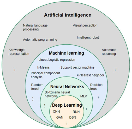
Image credit: zhuanlan.Zhihu.com
There is a wide variety of deep learning libraries, but currently, you will find that many applications use one of the following:
- Tensorflow. TensorFlow is a free and open-source software library for machine learning and artificial intelligence. It can be used across a range of tasks but has a particular focus on training and inference of deep neural networks. TensorFlow was developed by the Google Brain team for internal Google use in research and production.
- Keras. Keras is an open-source software library that provides a Python interface for artificial neural networks. Keras acts as an interface for the TensorFlow library.
- Pytorch. PyTorch is a machine learning framework based on the Torch library, used for applications such as computer vision and natural language processing, originally developed by Meta AI and now part of the Linux Foundation umbrella. It is free and open-source software released under the modified BSD license.
- fast.ai. fast.ai is a non-profit research group focused on deep learning and artificial intelligence. It was founded in 2016 by Jeremy Howard and Rachel Thomas with the goal of democratizing deep learning.
- Apache MXNet. Apache MXNet is an open-source deep learning software framework, used to train and deploy deep neural networks. It is scalable, allowing for fast model training and supports a flexible programming model and multiple programming languages. The MXNet library is portable and can scale to multiple GPUs as well as multiple machines. It was co-developed by Carlos Guestrin at University of Washington.
- Caffe. Caffe is a deep learning framework, originally developed at the University of California, Berkeley. It is open source, under a BSD license. It is written in C++, with a Python interface.
- Google JAX. Google JAX is a machine learning framework for transforming numerical functions. It is described as bringing together a modified version of autograd and TensorFlow's XLA. It is designed to follow the structure and workflow of NumPy as closely as possible and works with various existing frameworks such as TensorFlow and PyTorch.
TensorFlow has become the foremost popular Deep Learning framework. It supports multiple languages for creating deep learning models. Researchers of the Google brain team have developed this with the machine intelligence organization of Google.
The latest version is Tensorflow 2.0.
You can find all the Tensorflow documentation and learning resources in this link.
More Tensorflow resources:
PyTorch is the prime software tool after tensorflow. It operates with a dynamically updated graph. It supports data parallelism and distributed learning models. PyTorch is better for small projects and prototyping.
The latest version is Pytorch 1.13.
You can find the Pytorch Learning Resources in this link.
More Pytorch resources:
fast.ai is a deep learning library for Python that is designed to be easy to use and powerful. It is built on top of PyTorch, and provides a high-level API that makes it easy to train and deploy deep learning models. fast.ai is used by a wide range of people, from researchers to data scientists to engineers. It is a popular choice for both beginners and experienced users.
Here are some of the things that fast.ai can be used for:
- Image classification
- Natural language processing
- Speech recognition
- Object detection
- Machine translation
- Recommender systems
- Medical image analysis
- Financial forecasting
- And much more!
fast.ai is a powerful tool that can be used to solve a wide range of problems. It is easy to learn and use, and it is constantly being updated with new features and improvements. If you are interested in deep learning, fast.ai is a great place to start.
More fast.ai resources:
- Practical Deep Learning
- fast.ai software documentation
- fast.ai Blog
- fast.ai forum
- fast.ai GitHub repository
MXNet is another high-level library like Keras. It supports distributed computing. MXNet allows users to train networks over multiple GPU/CPU machines.
The latest version is MXNet 1.9.1.
More Apache MXNet resources:
Neural Networks are used in every field: data science, cybersecurity, aviation, education, health sciences, manufacturing, geosciences, and finances, to mention a few.
-
Speech recognition. Speech recognition is an interdisciplinary subfield of computer science and computational linguistics that develops methodologies and technologies that enable the recognition and translation of spoken language into text by computers with the main benefit of searchability.
-
Facial recognition systems. A facial recognition system is a technology capable of matching a human face from a digital image or a video frame against a database of faces. Such a system is typically employed to authenticate users through ID verification services and works by pinpointing and measuring facial features from a given image. Development began on similar systems in the 1960s, beginning as a form of computer application. Since their inception, facial recognition systems have seen wider uses in recent times on smartphones and in other forms of technology, such as robotics.
-
Optical character recognition. Optical character recognition or optical character reader is the electronic or mechanical conversion of images of typed, handwritten, or printed text into machine-encoded text, whether from a scanned document, a photo of a document, a scene photo, or from subtitle text superimposed on an image.
-
Signature recognition. Signature recognition is an example of behavioral biometrics that identifies a person based on their handwriting. It can be operated in two different ways: Static: In this mode, users write their signature on paper, and after the writing is complete, it is digitized through an optical scanner or a camera to turn the signature image into bits
-
Machine translation. Machine translation, sometimes referred to by the abbreviation MT, is a sub-field of computational linguistics that investigates the use of software to translate text or speech from one language to another.
-
Natural language generation. Natural language generation is a software process that produces natural language output. In one of the most widely-cited surveys of NLG methods, NLG is characterized as "the subfield of artificial intelligence and computational linguistics that is concerned with the construction of computer systems that can produce understandable texts in English or other human languages from some underlying non-linguistic representation of information".
-
Text-to-image. A text-to-image model is a machine learning model which takes as input a natural language description and produces an image matching that description. Such models began to be developed in the mid-2010s, as a result of advances in deep neural networks.
-
Automatic summarization. Automatic summarization is the process of shortening a set of data computationally, to create a subset that represents the most important or relevant information within the original content. In addition to text, images and videos can also be summarized. (Examples: Scholarcy, Wordtune, genei, ... )
-
Behavioral analytics. Behavioral analysis focuses on understanding how consumers act and why enabling accurate predictions about how they are likely to act in the future. It enables marketers to make the right offers to the right consumer segments at the right time. Behavioral analytics can be useful for authentication and security purposes.
-
Object Detection. Object detection is a computer technology related to computer vision and image processing that deals with detecting instances of semantic objects of a certain class in digital images and videos. Well-researched domains of object detection include face detection and pedestrian detection. Object detection has applications in many areas of computer vision, including image retrieval and video surveillance.
-
Image segmentation. In digital image processing and computer vision, image segmentation is the process of partitioning a digital image into multiple image segments, also known as image regions or image objects. The goal of segmentation is to simplify and/or change the representation of an image into something that is more meaningful and easier to analyze.
-
Gesture recognition. Gesture recognition is a topic in computer science and language technology with the goal of interpreting human gestures via mathematical algorithms. It is a subdiscipline of computer vision. Gestures can originate from any bodily motion or state but commonly originate from the face or hand.
- Stable Diffusion. AI image generation.
- HuggingFace | Tasks Library | Models
- Transformers. A transformer is a deep learning model that adopts the mechanism of self-attention, differentially weighting the significance of each part of the input data. It is used primarily in the fields of natural language processing and computer vision. Examples: Google's Bidirectional Encoder Representations from Transformers (BERT), OpenAI'sGenerative Pre-trained Transformer 3 (GPT-3), Google's Language Model for Dialogue Applications (LaMDA)
- Computer Vision - PWC. Computer vision is an interdisciplinary scientific field that deals with how computers can gain high-level understanding from digital images or videos. From the perspective of engineering, it seeks to understand and automate tasks that the human visual system can do.
- Natural Language Processing - PWC. Natural language processing is a subfield of linguistics, computer science, and artificial intelligence concerned with the interactions between computers and human language, in particular how to program computers to process and analyze large amounts of natural language data.
- Reinforcement Learning - PWC. Reinforcement learning is an area of machine learning concerned with how intelligent agents ought to take actions in an environment in order to maximize the notion of cumulative reward. Reinforcement learning is one of three basic machine learning paradigms, alongside supervised learning and unsupervised learning.
- Audio - PWC. Audio signal processing is a subfield of signal processing that is concerned with the electronic manipulation of audio signals. Audio signals are electronic representations of sound waves—longitudinal waves which travel through the air, consisting of compressions and rarefactions.
- Sequential - PWC. Sequential pattern mining is a topic of data mining concerned with finding statistically relevant patterns between data examples where the values are delivered in a sequence. It is usually presumed that the values are discrete, and thus time series mining is closely related, but usually considered a different activity.
- Graphs - PWC. In computer science, a graph is an abstract data type that is meant to implement the undirected graph and directed graph concepts from the field of graph theory within mathematics. A graph data structure consists of a finite set of vertices, together with a set of unordered pairs of these vertices for an undirected graph or a set of ordered pairs for a directed graph.
- Artificial Neural Networks Explained | Jupyter Notebook. Aegeus Zerium.
- A Visual and Interactive Guide to the Basics of Neural Networks. Jay Alammar.
- Deep Learning. Wikipedia.
- Deep Learning. IBM Cloud Education.
- Deep Learning Methods. Wolfram Research.
- Dive into Deep Learning. Aston Zhang, Zachary C. Lipton, Mu Li, and Alexander J. Smola.
- Neural Network 101. NeuralNetwork101.com.
- PapersWithCode. Free and open resource with Machine Learning papers, code, datasets, methods, and evaluation tables.
- Python Machine Learning, 3rd. Ed., Sebastian Raschka, and Vahid Mirjalili.
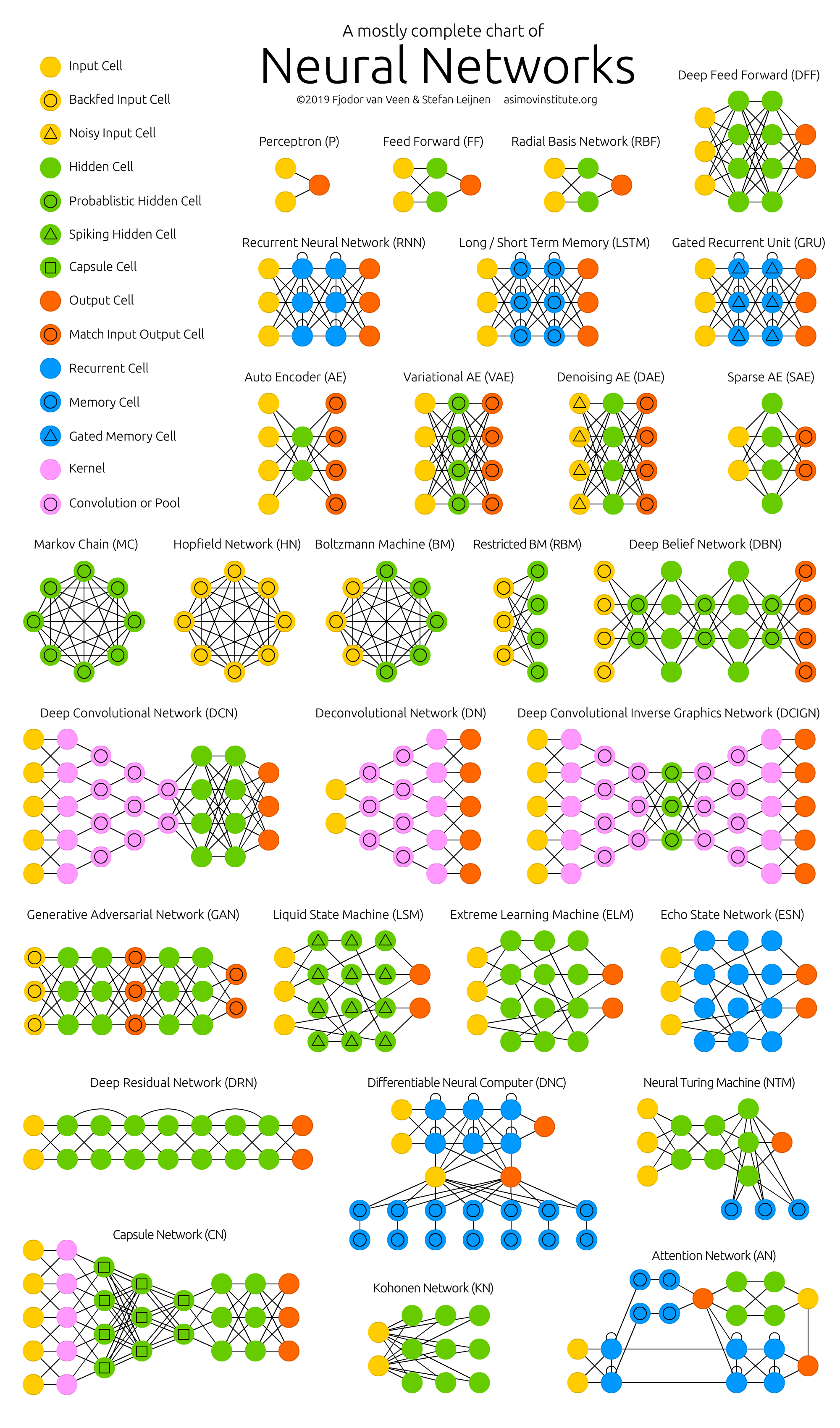
- The Neural Network Zoo. Fjodor Van Veen, The Asimov Institute.
- The Principles of Deep Learning Theory. Roberts, Daniel A. and Yaida, Sho and Hanin, Boris.
- Three Perspectives on Deep Learning. Sam Greydanus.
- Understanding Deep Learning. Simon J.D. Prince.
- CS-229 Machine Learning. Shervine Amidi, Stanford University; Afshine Amidi, MIT.
- CS-230 Deep Learning. Shervine Amidi, Stanford University; Afshine Amidi, MIT.
- A guide to machine learning for biologists. Greener, J. G., Kandathil, S. M., Moffat, L., & Jones, D. T. (2022). Nature Reviews Molecular Cell Biology, 23(1), 40-55.
- A primer on deep learning in genomics. Zou, J., Huss, M., Abid, A., Mohammadi, P., Torkamani, A., & Telenti, A. (2019). Nature genetics, 51(1), 12-18.
- Deep learning for plant genomics and crop improvement. Wang, H., Cimen, E., Singh, N., & Buckler, E. (2020). Current opinion in plant biology, 54, 34-41.
Created: 11/25/2022
Updated: 05/25/2022
Carlos Lizárraga

The University of Arizona. Data Science Institute, 2022.
