An Overview of Machine Learning Algorithms - clizarraga-UAD7/Workshops GitHub Wiki

Image credit: J.P.Morgan Macro QDS
Please see: A Python for Data Science Refresher
- Supervised Learning. Supervised model algorithms learn relationships using a dataset that already contains the label that the model should predict. However, they can only recognize and learn structures that are contained in the training data.
There are two main types of supervised learning problems: they are classification which involves predicting a class label and regression which involves predicting a numerical value.
- Classification: Supervised learning problem that involves predicting a class label.
- Regression: Supervised learning problem that involves predicting a numerical label.
Both classification and regression problems may have one or more input variables and input variables may be any data type, such as numerical or categorical.
📎 Examples:

Image credit: Jorge Leonel - Medium
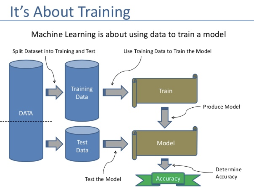
Image credit: Jorge Leonel - Medium
📎 Examples:
-
Credit card fraud detection. The input data would be the features of a credit card transaction, such as the amount of the transaction, the type of card, and the location of the transaction. The output data would be whether the transaction is fraudulent or not. The model would be trained on a dataset of fraudulent and non-fraudulent transactions, and it would learn to predict whether a new transaction is fraudulent or not.
-
Classification of images. Using images that are already assigned to a class, they learn to recognize relationships that they can then apply to new images.
- Unsupervised Learning. Unsupervised model algorithms learn from a dataset, but one that does not yet have these labels. They try to recognize their own rules and structures in order to be able to classify the data into groups that have the same properties as far as possible.
There are many types of unsupervised learning, although there are two main problems that are often encountered by a practitioner: they are clustering which involves finding groups in the data and density estimation which involves summarizing the distribution of data.
- Clustering: Unsupervised learning problem that involves finding groups in data.
- Density Estimation: Unsupervised learning problem that involves summarizing the distribution of data.
Clustering and density estimation may be performed to learn about the patterns in the data.
Additional unsupervised methods may also be used, such as visualization which involves graphing or plotting data in different ways and projection methods which involves reducing the dimensionality of the data.
- Visualization: Unsupervised learning problem that involves creating plots of data.
- Projection: Unsupervised learning problem that involves creating lower-dimensional representations of data.
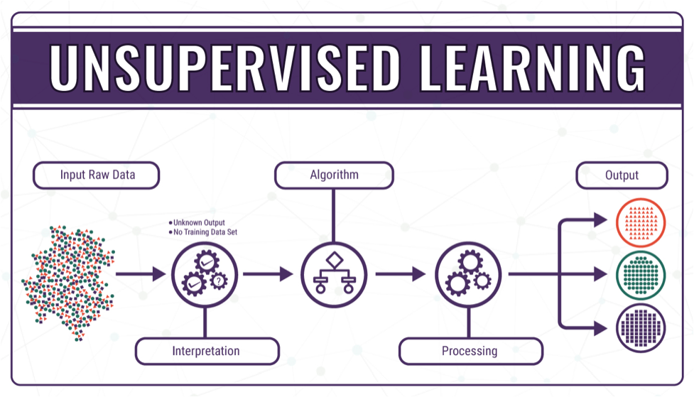
Image credit: Prerna Aditi - Medium
📎 Examples:
Customer segmentation is the process of grouping customers based on shared characteristics to understand their behavior and target marketing campaigns effectively.
Unsupervised learning can be used for customer segmentation, image clustering, and text clustering to gain insights from data.
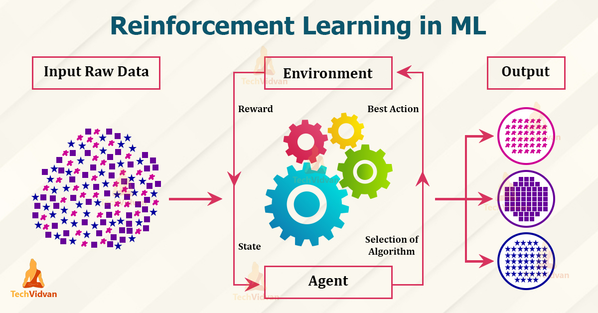
- Reinforcement Learning. The main difference is that the model does not need much data to train. It learns structures by being rewarded for desired behaviors and punished for bad ones.
📎 Examples:
The use of an environment means that there is no fixed training dataset, but rather a goal or set of goals that an agent is required to achieve, actions they may perform, and feedback about performance toward the goal.
Reinforcement learning is a powerful tool in machine learning that can be used to train agents to take actions that maximize rewards in complex environments, such as playing games, robotics, and stock trading.
The agent is given a reward for taking actions that lead to a desired outcome, and over time, the agent learns to take actions that maximize the reward through trial and error.
- Semi-Supervised Learning. It is a mixture of supervised learning and unsupervised learning. The model has a relatively small data set with labels available and a much larger data set with unlabeled data. The goal is to learn relationships from the small amount of labeled information and test those relationships in the unlabeled data set to learn from them.
📎 Examples:
Semi-supervised learning can be used to train a model to classify images by using a small dataset of labeled images and a large dataset of unlabeled images. This method helps the model to learn important features for classification and generalize to new images, making it a powerful tool for improving prediction accuracy with limited labeled data.
Semi-supervised learning can be used for text classification and speech recognition. It involves training a model on a small dataset of labeled data and a large dataset of unlabeled data to learn important features and generalize to new data.
- Self-Supervised Learning. It learns from the unlabeled sample data. It can be regarded as an intermediate form between supervised and unsupervised learning. It is based on an artificial neural network or other models such as a decision list. The model learns in two steps. First, the task is solved based on pseudo-labels which help to initialize the model parameters. Second, the actual task is performed with supervised or unsupervised learning. Self-supervised learning has produced promising results in recent years and has found practical application in audio processing and is being used by Facebook and others for speech recognition.
📎 Examples:
Self-supervised learning can be used to denoise images, such as faces, without the need for labeled data, improving prediction accuracy. The model would be trained on a dataset of noisy images of faces, and it would learn to predict the original, denoised image from the noisy image.
Self-supervised learning can be used for text completion and speech enhancement. Models are trained on datasets to predict the next word in a sentence or enhance speech with high accuracy. For example, a model could be trained to complete text in news articles. The model would be trained on a dataset of news articles, and it would learn to predict the next word in a sentence from the previous words in the sentence.
- Multi-Instance Learning. It is a type of supervised learning. Instead of receiving a set of instances that are individually labeled, the learner receives a set of labeled bags, each containing many instances. In the simple case of multiple-instance binary classification, a bag may be labeled negative if all the instances in it are negative. On the other hand, a bag is labeled positive if there is at least one instance in it that is positive. From a collection of labeled bags, the learner tries to either (i) induce a concept that will label individual instances correctly or (ii) learn how to label bags without inducing the concept.
📎 Examples:
Multiple instance learning can be used to classify images by training a model on a dataset of bags of instances. This approach can improve prediction accuracy for a variety of problems where data is in the form of bags of instances. For example, a model could be trained to classify text as spam or not spam. The model would be trained on a dataset of text, where each text is a bag of instances. The instances in a bag could be the words in the text, or they could be features extracted from the text.
Multiple instance learning can be used for text classification and drug discovery. The model is trained on a dataset of bags of instances, where the instances are related to each other, and the model learns to predict the label or activity based on the instances in the bag. The instances in a bag could be the chemical structure of the drug, or they could be features extracted from the chemical structure.
Statistical inference is the process of using data analysis to infer properties of an underlying distribution of probability.

- Concept Learning. Concept learning is a strategy that requires a learner to compare and contrast groups or categories that contain concept-relevant features with groups or categories that do not contain concept-relevant features.
📎 Examples:
Concept mapping can aid in feature selection for machine learning models, as demonstrated in the example of fruit classification. The concept map could be used to identify the most important concepts for fruit classification, such as color, shape, and size. The features that are related to those concepts, such as the red, green, and blue values of the pixels in the image, could be selected for the model.
Concept mapping can aid in visualizing data for machine learning models, allowing for identification of patterns and relationships to improve model accuracy. For example, a model could be trained to predict the price of a house. The concept map could be used to create a visual representation of the data, such as a scatter plot of the price of the house and the square footage of the house.
Concept mapping can aid in discovering knowledge from data for machine learning models, improving accuracy by identifying patterns and relationships in the data. Sure, here are some examples of concept mapping in machine learning:
- Feature selection. Concept mapping can be used to select features for machine learning models. The concept map can be used to identify the most important concepts for the task at hand, and the features that are related to those concepts can be selected for the model.
For example, a model could be trained to classify images of fruits. The concept map could be used to identify the most important concepts for fruit classification, such as color, shape, and size. The features that are related to those concepts, such as the red, green, and blue values of the pixels in the image, could be selected for the model.
- Data visualization. Concept mapping can be used to visualize data for machine learning models. The concept map can be used to create a visual representation of the data, which can help to identify patterns and relationships in the data.
For example, a model could be trained to predict the price of a house. The concept map could be used to create a visual representation of the data, such as a scatter plot of the price of the house and the square footage of the house. The patterns and relationships in the data can be identified from the visual representation, which can help to improve the accuracy of the model.
- Knowledge discovery. Concept mapping can be used to discover knowledge from data for machine learning models. The concept map can be used to identify patterns and relationships in the data, which can be used to discover new knowledge about the data.
For example, a model could be trained to predict the risk of a patient developing a disease. The concept map could be used to identify patterns and relationships in the data, such as the patient's age, gender, and medical history.
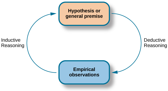
- Deductive Reasoning. It is the mental process of drawing deductive inferences. An inference is deductively valid if its conclusion follows logically from its premises, i.e. if it is impossible for the premises to be true and the conclusion to be false.
📎 Examples:
Deductive reasoning is used in machine learning for spam filtering and fraud detection based on a set of rules. These rules can be based on the content of the email, the sender's address, or other factors. For example, a rule might state that any email that contains the word "free" is likely to be spam.
Deductive reasoning can improve the accuracy of machine learning models in medical diagnosis by classifying patients based on a set of rules. For example, a rule might state that any patient who has a fever, cough, and shortness of breath is likely to have pneumonia.
- Transductive Learning. In logic, statistical inference, and supervised learning, transduction or transductive inference is reasoning from observed, specific (training) cases to specific (test) cases. In contrast, induction is reasoning from observed training cases to general rules, which are then applied to the test cases.
Image credit: Jason Brownlee - Machine Learning Mastery
📎 Examples:
Transductive learning trains a model to classify images using both labeled and unlabeled datasets. It is a powerful tool that improves prediction accuracy with limited labeled data.
For example, a model could be trained to classify images of cats and dogs. The model would be trained on a dataset of labeled images, such as images of cats with the label "cat" and images of dogs with the label "dog." The model would also be trained on a dataset of unlabeled images, such as images of animals that are not cats or dogs. Over time, the model would learn to classify images of cats and dogs with high accuracy.
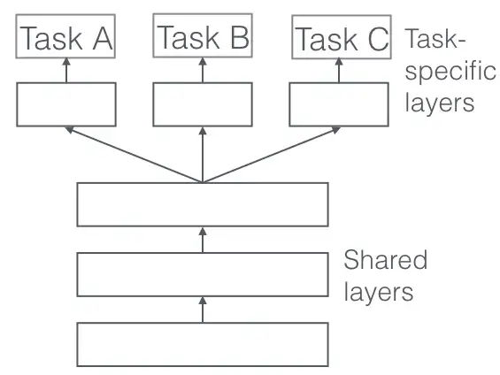
- Multi-Task Learning. Multiple learning tasks are solved at the same time while exploiting commonalities and differences across tasks.
📎 Examples:
Multi-task learning in machine learning can be used for image classification and object detection, where a model is trained to predict the label of an image and the location of objects within it.
Multi-task learning can train a model to classify text and analyze sentiment, improving accuracy over time.
Multi-task learning can train a model to recognize speech and model language by predicting the transcript of speech and the next word in text, leading to high accuracy in speech recognition and language modeling.
- Active Learning. It is the case when a learning algorithm can interactively query a user (or some other information source) to label new data points with the desired outputs.
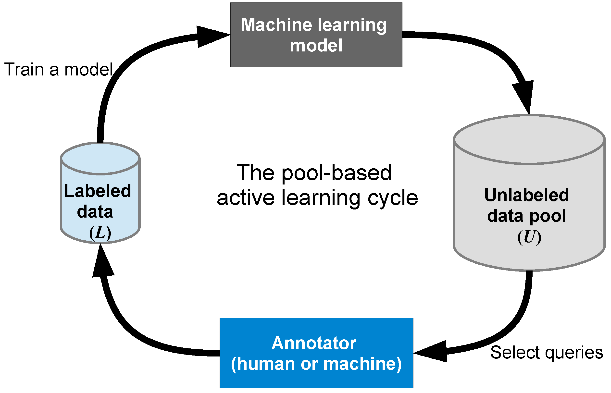
Image credit: Chris Zhu - Towards Data Science
📎 Examples:
Active learning can be used to train machine learning models for image classification by querying humans for labels of unlabeled images, resulting in improved accuracy.
Active learning can train a model to classify text by querying a human for labels of unlabeled text and retraining the model on the updated dataset until the desired accuracy is achieved. For instance, a model can be trained to classify emails as spam or not spam by learning from labeled and queried text.
Active learning can be used to train a model for medical diagnosis by querying a human for diagnoses of unlabeled data and retraining the model until desired accuracy is achieved.
Active learning in machine learning can improve accuracy, reduce labeling cost, increase efficiency, and improve interpretability. However, it can also be expensive, challenging with limited labeled data, and difficult to use with complex models or to improve interpretability.
- Transfer Learning. This type of learning focuses on storing knowledge gained while solving one problem and applying it to a different but related problem.
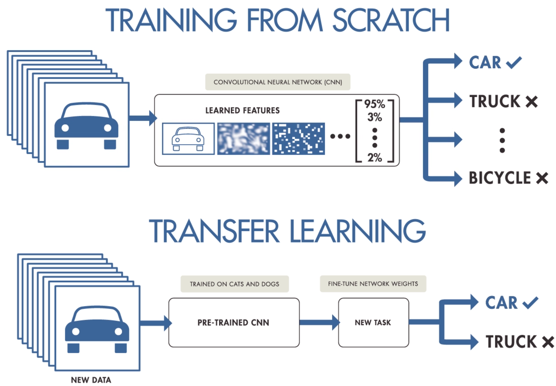
Image credit: Purnasai Gudikandula - Medium
📎 Examples:
Transfer learning can be used in machine learning for image classification, text classification or speech recognition, by training a pre-trained model on a large dataset of images and fine-tuning it on a smaller dataset specific to the task at hand.
Transfer learning can be used to train a model for by fine-tuning a pre-trained model on a smaller dataset specific to the task at hand.
Transfer learning in machine learning can improve accuracy, reduce training time, and increase model flexibility, but it also poses challenges such as data compatibility, model complexity, and interpretability.
- Ensemble Learning. This method uses multiple learning algorithms to obtain better predictive performance than could be obtained from any of the constituent learning algorithms alone.

📎 Examples:
Ensemble learning in machine learning includes methods like bagging, which creates multiple models from bootstrapped samples of training data and combines their predictions to create a final prediction.
Boosting is an ensemble learning method that creates multiple models in sequence by training on residuals of the previous model, and the predictions of the individual models are combined to create a final prediction.
Voting is an ensemble learning method that combines the predictions of multiple models to create a final prediction, with weights based on accuracy.
Ensemble learning can improve accuracy, reduce overfitting, and increase robustness of machine learning models, but challenges include model selection and computational complexity.

Classical Machine Learning Methods can be classified into 3 major paradigms:
In supervised learning, the algorithms construct a function from input-output examples, and then it will predict the outcome given an unlabeled input.
Example problems are classification and regression analysis.
The most widely used learning algorithms are:
- Support-vector machines (Visual example)
- Linear regression (Visual example)
- Logistic regression
- Naive Bayes
- Linear discriminant analysis
- Decision trees (Visual example)
- Random Forest (Visual example)
- K-nearest neighbor algorithm
- Neural networks (Multilayer perceptron) (Visual example)
- Similarity learning
In Unsupervised Learning, the algorithms learn to detect regularity or patterns from untagged data.
Some of the most common algorithms used in unsupervised learning include:
- Clustering,
- Anomaly detection,
- Approaches for learning latent variable models.
Each approach uses several methods as follows:
-
Clustering methods include: hierarchical clustering, k-means, mixture models, DBSCAN, and OPTICS algorithm
-
Anomaly detection methods include: Local Outlier Factor, and Isolation Forest
-
Approaches for learning latent variable models such as Expectation–maximization algorithm (EM), Method of moments, and Blind signal separation techniques (Principal component analysis, Independent component analysis, Non-negative matrix factorization, Singular value decomposition) (Visual example of PCA)
- Weak Supervised Learning. This process lands between supervised and unsupervised learning methods. It occurs when there is only a noisy, limited, or imprecise set of data used in supervised training for labeling large amounts of training data.
Reinforcement learning (RL) is an area of machine learning concerned with how intelligent agents ought to take actions in an environment in order to maximize the notion of cumulative reward.
Examples of reinforcement learning algorithms:
- Awesome Machine Learning Visualizations (Github). Mohamed Kedir Noordeen.

Scikit-learn is a machine-learning library for Python. It features various classification, regression analysis, cluster analysis, and efficient tools for data mining and data analysis. It’s built on NumPy, SciPy, and Matplotlib.

- Loading the data
Load the as a standard Pandas dataframe.
import pandas as pd
df = pd.read_csv(filename)
- Split data: Train & Test
Split the dataset into training and test sets for both the X and y variables.
Function: sklearn.model_selection.train_test_split
from sklearn.model_selection import train_test_split
X_train,X_test,y_train,y_test = train_test_split(X, y, test_size=0.2, random_state = 0)
- Preprocessing the data
Getting the data ready before the model is fitted.
Standardize the features by removing the mean and scaling to unit variance.
Function: sklearn.preprocessing.StandardScaler
from sklearn.preprocessing import StandardScaler
scaler = StandardScaler().fit(X_train)
standarized_X = scaler.transform(X_train)
standarized_X_test = scaler.transform(X_test)
Each sample with at least one non-zero component is rescaled independently of other samples so that its norm equals one.
Function: sklearn.preprocessing.Normalizer
from sklearn.preprocessing import Normalizer
scaler = Normalizer().fit(X_train)
normalized_X = scaler.transform(X_train)
normalized_X_test = scaler.transform(X_test)
Binarize data (set feature values to 0 or 1) according to a threshold.
Function: sklearn.preprocessing.Binarizer
from sklearn.preprocessing import Binarizer
binarizer = Binarizer(threshold = 0.0).fit(X)
binary_X = binarizer.transform(X_test)
Encode’s target labels with values between 0 and n_classes-1.
Function: sklearn.preprocessing.LabelEncoder
from sklearn import preprocessing
le = preprocessing.LabelEncoder()
le.fit_transform(X_train)
Imputation transformer for completing missing values.
Function: sklearn.impute.SimpleImputer
from sklearn.impute import SimpleImputer
imp = SimpleImputer(missing_values = 0, strategy = 'mean')
imp.fit_transform(X_train)
Generate a new feature matrix consisting of all polynomial combinations of the features with degrees less than or equal to the specified degree.
Function: sklearn.preprocessing.PolynomialFeatures
from sklearn.preprocessing import PolynomialFeatures
poly = PolynomialFeatures(5)
poly.fit_transform(X)
- Create the model
Creation of various supervised and unsupervised learning models.
from sklearn.linear_model import LinearRegression
lr  = LinearRegression(normalize = True)
from sklearn.svm import SVC
svc = SVC(kernel = 'linear')
from sklearn.naive_bayes import GaussianNB
gnb = GaussianNB()
from sklearn import neighbors
knn = neighbors.KNeighborsClassifier(n_neighbors = 5)
from sklearn.decomposition import PCA
pca = PCA(n_components = 0.95)
from sklearn.cluster import KMeans
k_means = KMeans(n_clusters = 3, random_state = 0)
- Fit the model
Fitting supervised and unsupervised learning models onto data.
- Supervised Learning
Fit the model to the data
lr.fit(X, y)
knn.fit(X_train,y_train)
svc.fit(X_train,y_train)
- Unsupervised Learning
Fit the model to the data
k_means.fit(X_train)
Fit the data, then transform it
pca_model = pca.fit_transform(X_train)
- Making predictions
Predicting test sets using trained models.
#Supervised Estimators
y_pred = lr.predict(X_test)

#Unsupervised Estimators
y_pred = k_means.predict(X_test)
y_pred = knn.predict_proba(X_test)
- Evaluating model performance
Various regression and classification metrics that determine how well a model performed on a test set.
knn.score(X_test,y_test)

from sklearn.metrics import accuracy_score
accuracy_score(y_test,y_pred)
from sklearn.metrics import classification_report
print(classification_report(y_test,y_pred))
from sklearn .metrics import confusion_matrix
print(confusion_matrix(y_test,y_pred))
from sklearn.metrics import mean_absolute_error
mean_absolute_error(y_test,y_pred)
from sklearn.metrics import mean_squared_error
mean_squared_error(y_test,y_pred)
from sklearn.metrics import r2_score
r2_score(y_test, y_pred)
from sklearn.metrics import adjusted_rand_score
adjusted_rand_score(y_test,y_pred)
from sklearn.metrics import homogeneity_score
homogeneity_score(y_test,y_pred)
from sklearn.metrics import v_measure_score
v_measure_score(y_test,y_pred)
Evaluate a score by cross-validation
from sklearn.model_selection import cross_val_score
print(cross_val_score(knn, X_train, y_train, cv=4))
- Model tuning
Finding correct parameter values that will maximize a model’s prediction accuracy.
A Grid Search is an exhaustive search over specified parameter values for an estimator. The example below attempts to find the right amount of clusters to specify for knn to maximize the model’s accuracy.
from sklearn.model_selection import GridSearchCV

params = {'n_neighbors': np.arange(1,3), 'metric':['euclidean','cityblock']}

grid = GridSearchCV(estimator = knn, param_grid = params)
grid.fit(X_train, y_train)
print(grid.best_score_)
print(grid.best_estimator_.n_neighbors)
Randomized search on hyperparameters. In contrast to Grid Search, not all parameter values are tried out, but rather a fixed number of parameter settings is sampled from the specified distributions. The number of parameter settings that are tried is given by n_iter.
from sklearn.model_selection import RandomizedSearchCV
params = {'n_neighbors':range(1,5), 'weights':['uniform','distance']}
rsearch = RandomizedSearchCV(estimator = knn, param_distributions = params, cv = 4, n_iter = 8, random_state = 5)
rseach.fit(X_train, y_train)
print(rsearch.best_score_)
- Machine Learning. Wikipedia.
- Machine Learning Tutorial. TechVidvan.
- ML Papers Explained. DAIR.AI (Democratizing Artificial Intelligence Research, Education, and Technologies).
- Scikit-Learn Library.
- What is Scikit-Learn. DatabaseCamp.de.
- Introduction to Machine Learning.
Created: 11/14/2022
Last update: 05/23/2023
Carlos Lizárraga

