openCV_히스토그램 - chloe73/openCV GitHub Wiki
히스토그램이란 도수 분포표 중 하나로 데이터의 분포를 몇 개의 구간으로 나누고 각 구간에 속하는 데이터를 시각적으로 표현한 막대그래프입니다.
이미지에서 사용하는 히스토그램은 X 축을 픽셀의 값으로 사용하고 Y 축을 해당 픽셀의 개수로 표현합니다.
이미지의 픽셀값을 히스토그램으로 표현하면 이미지의 특성을 쉽게 확인할 수 있습니다.
히스토그램은 다음과 같은 세 가지의 중요한 요소를 갖고 있습니다.
-
빈도 수(BINS): 히스토그램 그래프의 X 축 간격 -
차원 수(DIMS): 히스토그램을 분석할 이미지의 차원 -
범위(RANGE): 히스토그램 그래프의 X 축 범위
빈도 수는 히스토그램의 X 축 간격입니다. 픽셀값의 범위는 0~255로 총 256개의 범위를 갖고 있으며, 빈도 수의 값이 8이라면 0 ~ 7, 8 ~ 15, …, 248 ~ 255의 범위로 총 32개의 막대가 생성됩니다.
차원 수는 이미지에서 분석하고자 하는 색상 차원을 의미합니다. 그레이스케일은 단일 채널이므로 하나의 차원에 대해 분석할 수 있고 색상 이미지는 다중 채널이므로 세 개 이상의 차원에 대해 분석할 수 있습니다.
범위는 이미지에서 측정하려는 픽셀값의 범위로서, 특정 픽셀값 영역에 대해서만 분석하게 하는 데 사용됩니다.
import cv2
from matplotlib import pyplot as plt

imgFile = "resource/img.jpg" # 파일 위치 저장
img = cv2.imread(imgFile,0)

plt.hist(img.ravel(), 256, [0,256]);
plt.show()
[결과]

# ========== 히스토그램 균일화(평활화) : Histogram Equalization ===========
import cv2
import numpy as np
from matplotlib import pyplot as plt

imgFile = "resource/111.jpg" # 파일 위치 저장
img = cv2.imread(imgFile, 0)

hist, bins = np.histogram(img.ravel(), 256,[0,256]) # 히스토그램 구하기
cdf = hist.cumsum()  # numpy 배열을 1차원으로 하고 더한 값을 누적하여 배열 생성

cdf_m = np.ma.masked_equal(cdf, 0)  # cdf에서 값이 0인 부분을 mask하여 제외 처리

cdf_m = (cdf_m - cdf_m.min()) * 255 / (cdf_m.max() - cdf_m.min())  # 여기가 균일화 방정식

cdf = np.ma.filled(cdf_m, 0).astype('uint8')  # mask로 제외했던 0값을 복원

img2 = cdf[img]

cv2.imshow('Equalization', img2)

cv2.waitKey(0)

cv2.destroyAllWindows()# Script is based on https://github.com/richzhang/colorization/blob/master/colorization/colorize.py
# To download the caffemodel and the prototxt, see: https://github.com/richzhang/colorization/tree/master/colorization/models
# To download pts_in_hull.npy, see: https://github.com/richzhang/colorization/blob/master/colorization/resources/pts_in_hull.npy
import numpy as np
import cv2 as cv
from matplotlib import pyplot as plt
W_in = 224
H_in = 224
prototxt = "colorization_deploy_v2.prototxt.txt"
caffemodel = "colorization_release_v2.caffemodel"
kernel = "pts_in_hull.npy"
input = "test1.jpg"
# Select desired model
net = cv.dnn.readNetFromCaffe(prototxt, caffemodel)
pts_in_hull = np.load(kernel) # load cluster centers
# populate cluster centers as 1x1 convolution kernel
pts_in_hull = pts_in_hull.transpose().reshape(2, 313, 1, 1)
net.getLayer(net.getLayerId('class8_ab')).blobs = [pts_in_hull.astype(np.float32)]
net.getLayer(net.getLayerId('conv8_313_rh')).blobs = [np.full([1, 313], 2.606, np.float32)]
if input:
cap = cv.VideoCapture(input)
else:
cap = cv.VideoCapture(0)
width = int(cap.get(cv.CAP_PROP_FRAME_WIDTH))
height = int(cap.get(cv.CAP_PROP_FRAME_HEIGHT))
imshowSize = (width, height)
hasFrame, frame = cap.read()
img_rgb = (frame[:,:,[2, 1, 0]] * 1.0 / 255).astype(np.float32)
img_lab = cv.cvtColor(img_rgb, cv.COLOR_RGB2Lab)
img_l = img_lab[:,:,0] # pull out L channel
(H_orig,W_orig) = img_rgb.shape[:2] # original image size
# resize image to network input size
img_rs = cv.resize(img_rgb, (W_in, H_in)) # resize image to network input size
img_lab_rs = cv.cvtColor(img_rs, cv.COLOR_RGB2Lab)
img_l_rs = img_lab_rs[:,:,0]
img_l_rs -= 50 # subtract 50 for mean-centering
net.setInput(cv.dnn.blobFromImage(img_l_rs))
ab_dec = net.forward()[0,:,:,:].transpose((1,2,0)) # this is our result
(H_out,W_out) = ab_dec.shape[:2]
ab_dec_us = cv.resize(ab_dec, (W_orig, H_orig))
img_lab_out = np.concatenate((img_l[:,:,np.newaxis],ab_dec_us),axis=2) # concatenate with original image L
img_rgb_out = np.clip(cv.cvtColor(img_lab_out, cv.COLOR_Lab2RGB), 0, 1)
frame = cv.resize(frame, imshowSize)
plt.rcParams['figure.figsize'] = [13, 13]
plt.subplot(2, 2, 1)
plt.imshow(frame)
plt.axis("off")
plt.title("Origin", fontsize=18)
plt.subplot(2, 2, 2)
gray = cv.cvtColor(frame, cv.COLOR_BGR2GRAY)
plt.imshow(gray, cmap='gray')
plt.axis("off")
plt.title("Gray scale", fontsize=18)
plt.subplot(2, 2, 3)
plt.imshow(img_rgb_out)
plt.axis("off")
plt.title("Colorization", fontsize=18)
plt.imsave("colorization.jpg", img_rgb_out)
img = cv.imread("colorization.jpg")
color = ('b', 'r', 'g')
plt.subplot(2, 2, 4)
for i, c in enumerate(color):
hist_c = cv.calcHist([img], [i], None, [256], [0, 256])
plt.plot(hist_c, color=c)
plt.xlim([0, 256])
plt.grid()
plt.title("Histogram color", fontsize=18)
plt.show()#include "opencv2/objdetect/objdetect.hpp"
#include "opencv2/highgui/highgui.hpp"
#include "opencv2/imgproc/imgproc.hpp"
#include <iostream>
using namespace std;
using namespace cv;
int main()
{
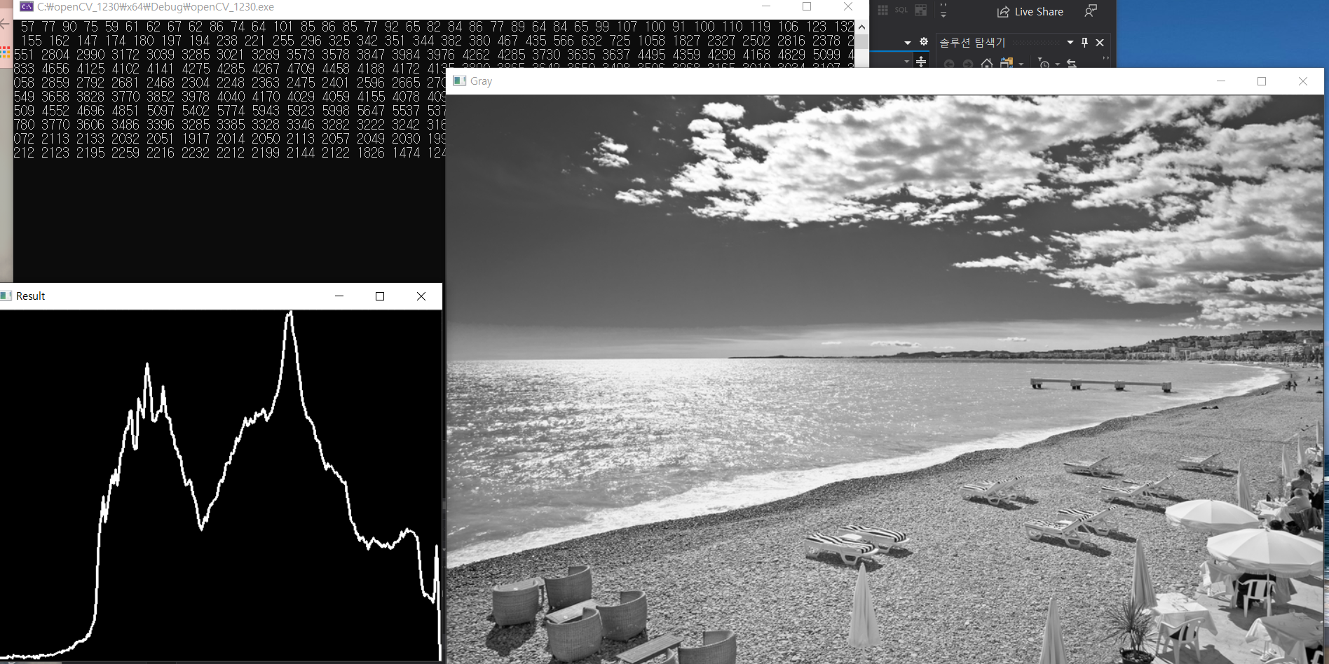
cv::Mat gray = cv::imread("111.jpg", IMREAD_GRAYSCALE);
cv::namedWindow("Gray", 1);
cv::imshow("Gray", gray);
/// Initialize parameters
int histSize = 256; // bin size
float range[] = { 0, 255 };
const float* ranges[] = { range };
/// Calculate histogram
cv::MatND hist;
cv::calcHist(&gray, 1, 0, cv::Mat(), hist, 1, &histSize, ranges, true, false);
/// Show the calculated histogram in command window
double total;
total = gray.rows * gray.cols;
for (int h = 0; h < histSize; h++)
{
float binVal = hist.at<float>(h);
std::cout << " " << binVal;
}
/// Plot the histogram
int hist_w = 512;
int hist_h = 400;
int bin_w = cvRound((double)hist_w / histSize);
cv::Mat histImage(hist_h, hist_w, CV_8UC1, cv::Scalar(0, 0, 0));
cv::normalize(hist, hist, 0, histImage.rows, NORM_MINMAX, -1, cv::Mat());
for (int i = 1; i < histSize; i++)
{
line(histImage, cv::Point(bin_w * (i - 1), hist_h - cvRound(hist.at<float>(i - 1))),
cv::Point(bin_w * (i), hist_h - cvRound(hist.at<float>(i))),
cv::Scalar(255, 0, 0), 2, 8, 0);
}
cv::namedWindow("Result", 1);
cv::imshow("Result", histImage);
cv::waitKey(0);
return 0;
}