Example 8 : Transient flow around an Ahmed body - chaos-polymtl/lethe GitHub Wiki

In this example, a flow is passing across a fixed Ahmed body (simplified version of a car, classical benchmark for aerodynamic simulation tools). The velocity profile of the flow is simulated. The parameter file used is ahmed.prm.

The following schematic describes the simulation.

• bc = 0 (No slip boundary condition)
• bc = 1 (u = 1; flow in the x-direction)
• bc = 2 (Slip boundary condition)

The basic geometry for the Ahmed body is given below, as defined in Ahmed and al., 1984, with all measures in mm.

Geometry parameters can be adapted in the "Parameters" section of the .geo file, as shown below. Namely the step parameter phi can be easily adapted.

//===========================================================================
//Parameters
//===========================================================================
unit = 1000; //length unit : 1 -> mm ; 1000 -> m
phi = 20; //angle at rear, variable
esf = 2.0e-1; //element size factor, used in the free quad mesh

//Ahmed body basic geometry
L = 1044/unit;
H = 288/unit;
R = 100/unit;
Hw = 50/unit; //wheel height (height from the road)
Ls = 222/unit; //slope length

//Fluid domain
xmin = -500/unit;
ymin = -Hw;
xmax = 2500/unit;
ymax = 1000/unit;

The initial mesh is built with Gmsh. It is defined as transfinite at the body boundary layer and between the body and the road, and free for the rest of the domain. The mesh is dynamically refined throughout the simulation.

The initial condition and boundary conditions are defined as in Example 3.

Time integration is defined by a 1st order backward differentiation (bdf1), for a 4 seconds simulation (time end) with a 0.01 second time step. The output path is defined to save obtained results in a sub-directory, as stated in Simulation Control:

# --------------------------------------------------
# Simulation Control
#---------------------------------------------------
subsection simulation control
  set method                  = bdf1
  set output frequency        = 1
  set output name             = ahmed-output
  set output path             = ./Re720/
  set time end                = 4
  set time step		      = 0.01
end

Ahmed body are typically studied considering a 60 m/s flow of air. Here, the flow speed is set to 1 (u = 1) so that the Reynolds number for the simulation (Re = uL/ν, with L the height of the Ahmed body) is varied through the kinematic viscosity ν:

#---------------------------------------------------
# Physical Properties
#---------------------------------------------------
subsection physical properties
    set kinematic viscosity         = 4e-4
end

The input mesh Ahmed_Body_20_2D.msh is in the same folder as the .prm file and is called with:

#---------------------------------------------------
# Mesh
#---------------------------------------------------
subsection mesh
    set type                 = gmsh
    set file name            = Ahmed_Body_20_2D.msh
end

The simulation is launched in the same folder as the .prm and .msh file, using the gls_navier_stokes_2d solver. To decrease simulation time, it is advised to run on multiple cpu, using mpirun:

  mpirun -np 6 ../../exe/bin/gls_navier_stokes_2d ahmed.prm

where here 6 is the number of cpu used.

Transient results are shown for three Re values:

Re	ν	Video	t = 0.5 s	t = 4 s
28.8	1e-2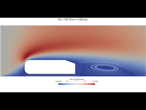
288	1e-3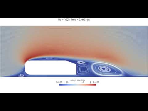
720	4e-4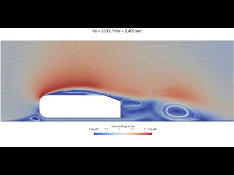

The mesh and processors load is adapted dynamically throughout the simulation, as shown below for Re = 720.

t = 0 s
t = 0.05 s
t = 4 s