ACKNOWLEDGEMENT

Tutorial Adapted from Ujaval Gandhi's QGIS Tutorials and Tips Orignally published at Quantum GIS (QGIS) Tutorials.

Download this tutorial from it's original source as a PDF in either A4 format of 'letter' format.

---

Here's another great resource! Check out Tim Sutton's The Free Quantum GIS Training Manual :"1. Lesson: Using Map Composer"

---

QGIS Print Composer allows you to take your GIS layers and package them to create maps. The tutorial shows how to create a map of Japan with standard map elements like north arrow, scale bar, legend and label.

Data used in this tutorial comes from the Natural Earth dataset - specifically the Natural Earth Quick Start Kit, which provides styled global layers. During the tutorial, we will load these layers directly into QGIS.

[Download the Natural Earth Quickstart Kit.]

Download and extract the Natural Earth Quick Start Kit data. Open QGIS. Click on File ‣ Open Project.

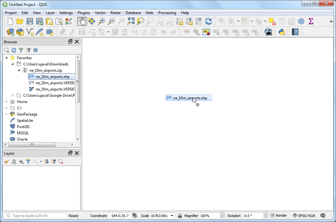
Browse to the directory when you had extracted the natural earth data. You should see a file named Natural_Earth_quick_start_for_QGIS.qgs. This is the project file that contains styled layers in QGIS Document format. Click Open.

You would see a lot of layers in the table of content and a styled world map in the QGIS canvas. If you see errors displayed at the top of the canvas, click on the cross to close it.

In this tutorial, we will make a map of Japan. Click the Zoom In button and draw a rectangle around Japan to zoom to the area.

Before we make a map suitable for printing, we need to choose an appropriate projection. This dataset comes in Geographic Coordinate System (GCS) where the units are degrees. This is not appropriate for a map where you want the distances to be in kilometers or miles. We need to use a Projected Coordinate System that minimizes distortions for our region of interest and has units in meters. Universal Transverse Mercator (UTM) is a decent choice for a projected coordinate system. It is also global, so it’s a good default that you can rely on and choose a UTM zone that contains your area of interest to minimize distortions for your region. In our case, we will use UTM Zone 54N. Click the CRS Status button at the bottom-right of the QGIS window.

Note: For Japan, Japan Plane Rectangular CS is a projected coordinate reference system (CRS) that is designed for minimum distortions. It is divided in 18 zones and if you are working for a smaller region in Japan, using this CRS will be better.

Check the Enable on-the-fly CRS Transformation box. Type Tokyo utm zone54n in the Filter search box. Once you see the results, select Tokyo / UTM Zone 54N - EPSG:3095. Click Apply.

Zoom and Pan to keep Japan at the center of your map canvas. At this point, you can check the box next to 10m_admin_0_map_units layer to turn off the labels from that layer.

Once you are centered around the area of interest, click on the New Print Composer button. It is also accessible by Project ‣ New Print Composer.

You will be prompted to enter a title for the composer. Enter ‘Japan map’ and click Ok.

In the Print Composer window, click on Zoom full to display the full extent of the Layout.

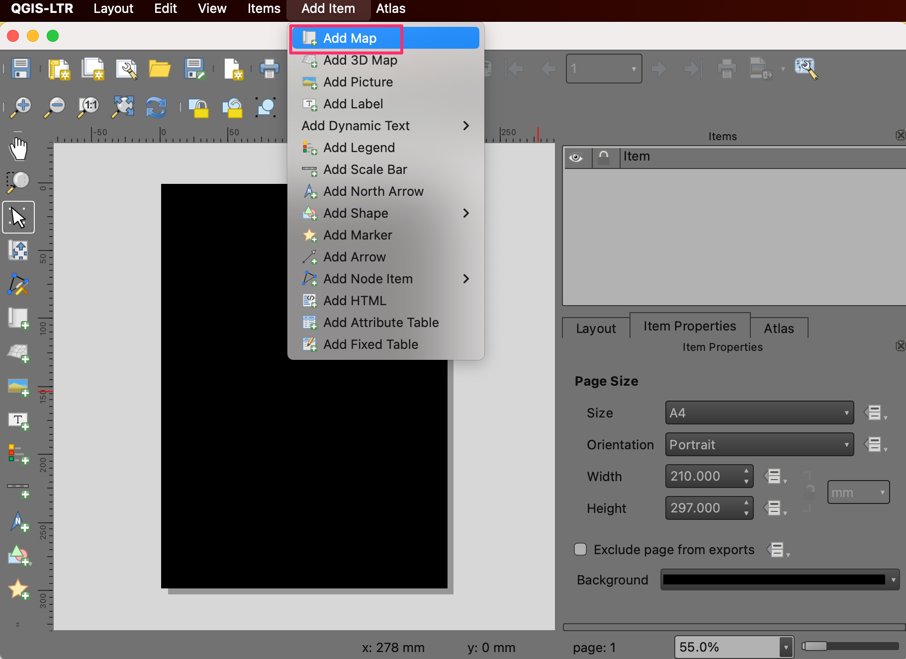
Now we would have to bring the map view that we see in the QGIS Canvas to this layer. Click on the Add Map button. This tool can also be access from Layout ‣ Add Map.

Once the Add Map button is active, hold the left mouse button and drag a rectangle where you want to insert the map.

You will see that the rectangle window will be rendered with the map from the main QGIS canvas. Since we want our map to be covering the full extent of the layout, drag the corners of the rectangle to the edges.

The rendered map may not be covering the full extent of our interest area. Click the Move item content button to pan the map in the window and center it in the composer.

Let us adjust the zoom level for the given map. Click on the Item Properties tab and enter 5000000 for Scale value.

Now we will add a North Arrow to the map. Print Composer comes with a nice collection of map-related images - including many types of North Arrows. Click Layout ‣ Add Image.

Holding your left mouse button, draw a rectangle on the top-right corner of the map canvas. On the right-hand panel, click on the Item Properties tab and expand the Search directories section and select the North Arrow image of your liking.

Next, scroll down below and un-check the Background option. This will make the image transparent.

You can drag the North Arrow and move it around in the composer window to a suitable position.

Now we will add a scale bar. Click on Layout ‣ Add Scalebar.

Click on the layout where you want the scalebar to appear. From the Item Properties tab, choose the Style that fit your requirement. You should also set the transparency by un-cecking the Background option.

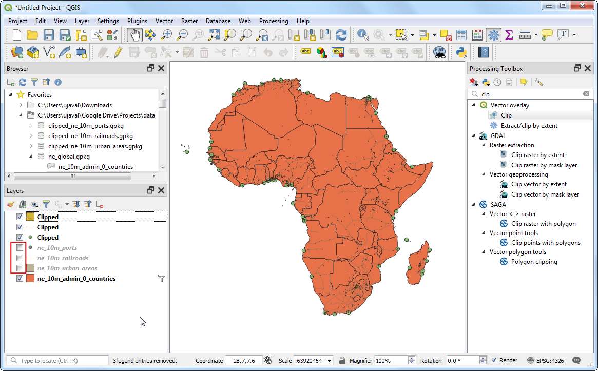
Now we will add a legend to the map. Click on Layout ‣ Add Legend.

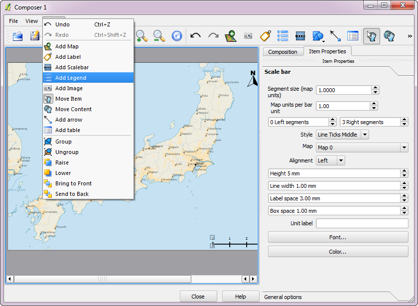
Click on the layout where you want the legend to appear. Since our layer list is huge, you will see a big box with all the layers appear. Click on the Item Properties tab and select the layers which we do not want in the legend. Click the - button to remove it from the legend.

For the purpose of this map, we will keep legend information only for the five layers as seen below.

Now time to label our map. Click on Layout ‣ Add Label.

Click on the map and draw a box where the label should be. In the Item Properties tab, expand the Label section and enter the text as shown below. We can enter the text as HTML as well. Check the box Render as Html so the composer will interpret the HTML tags.

Once you are satisfied with the map, you can export it as Image, PDF or SVG. For this tutorial, let’s export it as an image. Click Composer ‣ Export as Image.

Save the image in the format of your liking. Below is the exported PNG image.

This tutorials is copyright 2013, © Ujaval Gandhi. Mr. Gandhi's websites reserve no rights for the use and re-use of his tutorial. CCCS assumes his materials follow the same licensing as QGIS, namely Creative Commons Attribution-ShareAlike 3.0 (CC BY-SA).