Metropolis Monte Carlo - bertdupe/Matjes GitHub Wiki

Monte-Carlo (MC) algorithms are using random numbers. One of the most famous examples for a MC-simulation is the calculation of π, which you can find on the internet.

The goal of theoretical investigations using MC simulations of thermic systems is to calculate the expectation value of the energy and other thermodynamically quantities depending on temperature. In order to calculate this numerically, all possible states in a Boltzmann distribution have to be taken into account and the expectation value of your observable A is ⟨A⟩ = ∑ A_n e^-βE_n, where E_n is the energy of state X_n, A_n the value of A in state X_n and β=1/k_BT. This needs an enormous calculation effort.

The idea of MC simulations is to take only into account the states with the highest probability and have the highest contribution to the expectation value. But of course in doing so, one takes into account a certain uncertainty. At low temperature, the system stays most of the time in states of low energy. To consider this fact, the states are chosen with the Boltzmann probability p_n = 1/Z e^−βEn. If you have chosen your N states X_i like that (how to do it, see below), and calculate the value A_i of your observable in this state, you can calculate the estimated value with: A_i = ∑_i A_i.

To handle the problem of the choice of the Boltzmann distributed stated X_i, we use the Markov-process. Here, we generate a chain of states, where the transition from one state X_i to the state X_i+1 occurs with a certain transition probability p(X_i|X_i+1). The repetition of this Markov processes one gets the states X_i. The transition probability is not depending on other (former) states and does not change with time. p(X_i|X_I+1) has to fulfil the criteria of ergodicity, which makes sure, that every state can be reached by a chain of states. This is necessary to get the correct Boltzmann probabilities.

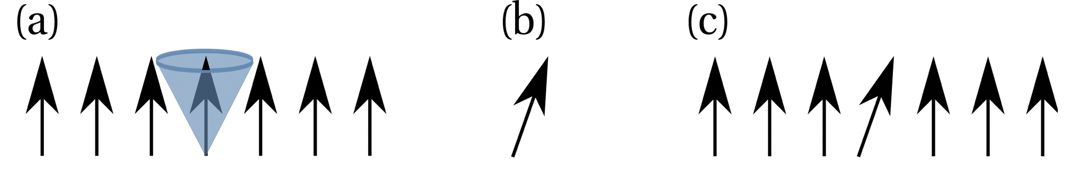
The Metropolis in configuration space enables the system to reach the next local energy minimum and a sampling of states in this minimum with a Boltzmann distribution. Here, the temperature is constant. The starting point of a MC simulation is a starting configuration of a spin structure, which can be random of given as the structure in Fig. (a). This state X_i has the energy E_i. In order to sample a chain of states, one choses a random spin, which is the one with the blue cone in Fig. (a). A new random orientation of the spin is then chosen (Fig. (b)) and exchanged with the transition probability p_relax = (X_i|X_I+i). This gives the new state X_i+1 as seen in Fig. (c) with an energy E_i+1. The probability p_relax = (X_i|X_i+1), that the spin is exchanged is given by p_relax =(X_i|X_i+1) = min(1,exp(−β∆E)), with ∆E = E_i+1- E_i. This means p_relax = (X_i|X_i+1) =1 if ∆E ≤ 0 and the energy of the new state X_i+1 is lower, and p_relax(X_i|X_i+1) =
e^−β∆E if ∆E > 0 and the energy of the new state X_i+1 is higher. The random orientation in Fig.(b) is chosen in a solid angle (blue shaded area in Fig. (a)) which yield an average exchange of the spin with a probability of 50%.

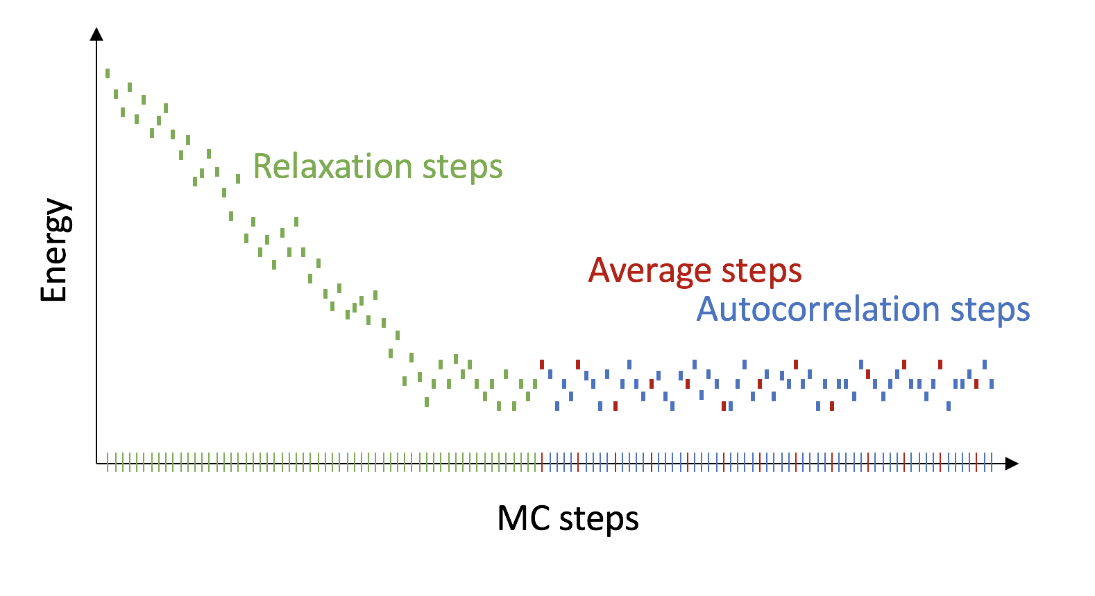
In practice, we distinguish between three different MC-steps. First, we relax the system to the next local energy minimum (relaxation steps). Then we sample our states (average steps), these are the X_i states from above. In between the average steps, we do autocorrelation steps. At the end, we average over the average steps.

• G. T. u. N. M. Newman, Mark EJ und Barkema. Monte Carlo methods in statistical physics, volume 13. Clarendon Press Oxford, (1999).
• Metropolis, A. Rosenbluth, Marshall Rosenbluth, A. Teller und Edward Teller: Equation of state calculation by fast computing machines. In: Journal of Chemical Physics. Band 21, 1953, S. 1087–1092
• T. Müller-Gronbach, E. Novak, and K. Ritter. Monte Carlo-Algorithmen. Springer- Verlag, (2012).