In order to describe the time dependent behaviour of magnetic moments in an effective field, we use the magnetization dynamics.

The dynamics of the magnetic moments is described with the Landau-Lifschitz (LL) or Landau-Lifschitz-Gilbert (LLG) equation, which are classical equations of motion based on a quantum mechanical spin system. The two equations differ in the describtion of the damping.

First, we will derive the classical LL(G) equation based on a quantum spin system for a magnetic moment M in an effective field H_i,eff, first without, then with damping. After we will show how thermal noise is included, then, a electric current is also considered within the spin transfer torque model.

The quantum mechanical equation of motion of the expectation value <S> of for a single spin S is given by

iℏ d/dt <S>(t) = <[S,Ĥ(S,t)]>,

where Ĥ(S,t) is the Hamilton operator.

We now apply the following aspects:

• For isotropic Hamiltonian holds: <[S,Ĥ]> = -iℏ <S ×∂ Ĥ/∂ S>
• Transition from quantum mechanical to classical equation of motion via Ehrenfest theorem: s = <S> and Ĥ = <H>
• Spin s and normalized magnetic moment m_i = μ_i /μ_s (μ_i: magnetic moment, μ_s: absolute value of μ_i) are connected via the gyromaganetic ratio: s_i = - M_i/γ = - μ_sm_i/γ (here, γ is the absolute value of the gyromagnetic ratio)
• For the effective magnetic field holds:H_i,eff = -(∂H / ∂ m_i)

This yields the LL equation without damping:

∂ m_i / ∂t = -γ/μ_s m_i × H_i,eff

So the magnetic moment m_i precesses around the effective field H_i,eff without changing its length.

The undamped LL equation can be extended by a phenomenological damping term which yiels the LL equation:

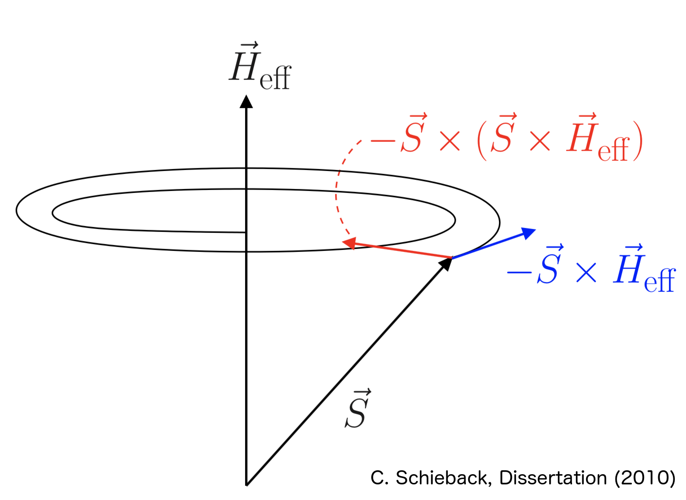
∂ m_i / ∂t = -γ/μ_s m_i × H_i,eff - α_LL/μ_s m_i × (m_i × H_i,eff)

The first term on the right side is the precession term (blue arrow in the following figure) the second term is the damping term (red arrow in the following figure) of the magnetic moments into the direction of the effective field.

For very large damping terms α_LL, the LL equation yield wrong results. Therefore, the LLG equation with another damping term can be used.

In order to avoid the wrong results for α_LL → ∞, the following Gilbert equation was proposed:

∂ m_i / ∂t = -γ/μ_s m_i × H_i,eff + α(m_i × ∂ m_i / ∂t) ,

where α is the Gilbert damping constant. The damping term is here dependent on the derivation of the magnetic moment with time (∂ m_i / ∂t).

It can be shown, that this equation can be transformed into a LL like form, which is then called the LLG equation:

∂ m_i / ∂t = - ^γ/_(1+α²)μs m_i × H_i,eff - ^γα/_(1+α²) m_i × (m_i × H_i,eff)

The difference between the LL and LLG equation is small for α<<1.

In the case of the LLG equation, the damping also influences the precession.

For small damping α² is negligible, and with α_LL = γα the LL and LLG are the same.

In the following, we will show, how the Gilbert equation is transformed to the LLG equation.

We start from Gilbert equation. Each side of the LLG must be multiplied by m_i ×. This gives:

m_i × ∂ m_i / ∂t = - γ/μ_s m_i × (m_i × H_i,eff) + αm_i × (m_i × ∂ m_i / ∂t),

This (m_i × ∂ m_i / ∂t ) can now be replaced in the Gilbert equation and all parts with a time derivative can be put on one side.

∂ m_i / ∂t - α²m_i × (m_i × ∂ m_i / ∂t)= - γ/μ_s (m_i × H_i,eff) - γα/μ_sm_i × (m_i × H_i,eff)

With the Leibniz rule for double cross product, m_i² = 1 and m_i × ∂ m_i / ∂t = 0 we yield the LLG equation.

To include the temperature, an effective noise ζ_i is included to the effective field H_i,eff. It follows the stochastic LLG equation:

∂ m_i / ∂t = - ^γ/_(1+α²)μs m_i × [H_i,eff+ζ_i] - ^γα/_(1+α²) m_i × (m_i × [H_i,eff+ζ_i])

The noise is a white noise with: <ζ_i> = 0.

When an eclectic current is applied to the magnetic system, the spins of the charge carriers interact with the local magnetization. Due to the conservation of angular momentum. This yield the spin transfer torque effect. A current can be used for example to move domain walls.

To include the effect of an electric current to the dynamic of an magnetic moment in an effective field, the LL, Gilbert and LLG equations can be extended with two terms, describing the adiabatic and non-adiabatic spin transfer torque effects.

The adiabatic spin torque effect describes the spin polarised current parallel to the change of the magnetization in a domain wall (for example both along the x-direction).

We assume in this adiabatic assumption, that the spins of the spin current are always along the local magnetization. As the local magnetization is changing along x, the x-component of the spin current density j_x is also changing in space. Due to the conservation of angular momentum, the local magnetization exerts a torque.

With the effective spin current u_x = j_x / M_s, the change of magnetization with time is for the general case (any direction of spin current)

∂m/∂t = - (u • ∇)S

The non-adiabatic spin transfer torque term describes the contributions of the spin transfer torque effect of the electron spins which are not parallel to the change of the magnetization in a domain wall. Its contribution to the LL equation is

∂m/∂t = β S × (u • ∇)S ,

where β is a non-adiabatic factor.

With the adiabatic and non-adiabatic term all spin orbit torque effects can be described.

The equations of motion which describe the dynamics of a magnetic moment in an effective field are now:

LL equation:

∂ m_i / ∂t = - γ/μ_s m_i × H_i,eff - α_LL/μ_s m_i × (m_i × H_i,eff) - (u • ∇)S + β_LL S × (u • ∇)S

Gilbert equation:

∂ m_i / ∂t = - γ/μ_s m_i × H_i,eff + α(m_i × ∂ m_i / ∂t) - (u • ∇)S + β S × (u • ∇)S ,

LLG equation:

∂ m_i / ∂t = - ^γ/_(1+α²)μs m_i × H_i,eff - ^γα/_(1+α²) m_i × (m_i × H_i,eff) - ^(1+βα)/_(1+α²) (u • ∇)S + ^(α-β)/_(1+α²) S × (u • ∇)S

The equations of motions are differential equations of the form:

d/dt x(t) = f(x(t),t) ,

where x is the unknown factor which can be a scalar or vectorial function. Such a differential equation can be displayed in the integral representation:

x(t) = x₀ + ∫_t0^t f(x(t'),t')dt' .

This differential equation can be solved (integrated) numerically.

To integrate the differential equation numerically, the time interval T = [t₀,t] has to be discretized to T = {t₀,t₁,...,t_N} with the time steps Δt = t_i+1,t_i.

In the following, different procedures to solve this equations are explained, where all of them only include the previous point x_i. They all follow the approximation instruction:

x_i+1 = x_i + Δt_i Φ

where Φ is the increment function. This instruction can be subdivided into:

Explicit one step process:
x_i+1 = x_i + Δt_i Φ(x_i,t_i) ,

where Φ(x_i,t_i) depends only on x_i and t_i.

Implicit one step process:
x_i+1 = x_i + Δt_i Φ(x_i,x_i+1,t_i) ,

where Φ(x_i,t_i) depends on x_i, t_i and also on the next (unknown) element x_i+1. Such implicit methods have to be solved for x_i+1 before it can be calculated.

More step process:
x_i+1 = x_i + Δt_i Φ(x₀,x₁,...,x_i,x_i+1,t_i) ,

where Φ(x_i,t_i) depends on x_i, t_i, the next (unknown) element x_i+1 and previous elements x₀,x₁,... .

The simplest method to integrate a differential equation is the Euler method. Here, the slope f(x_i) at position x_i, which is given by the differential equation is taken into account.
The explizit Euler method with Φ(x_i,t_i) = f(x_i) is:

x_i+1 = x_i + Δt_i f(x_i) .

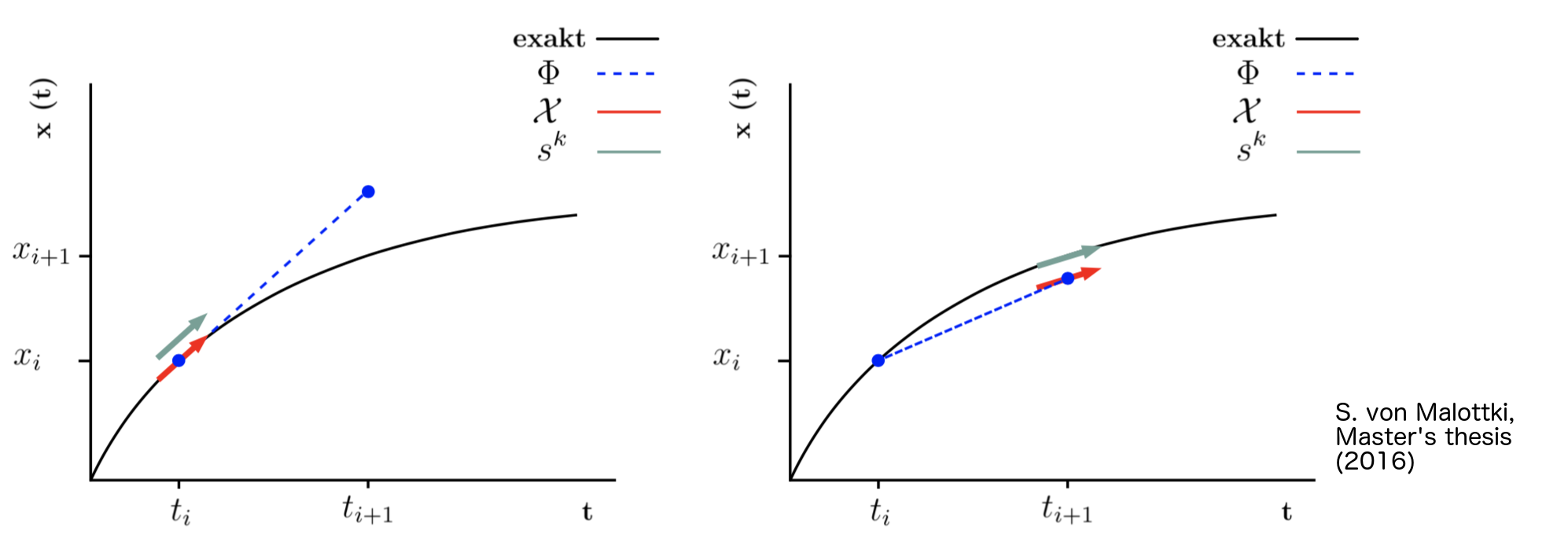
The problem of explizit one step processes is, that these methods can show an instability. Another possibility is the implicit Euler method with Φ(x_i,t_i) = f(x_i+1), which yield

x_i+1 = x_i + Δt_i f(x_i+1) .

A sketch of the two methods is shown in the following graph. On the left, the explicit Euler method, and on the right, the implicit Euler method is shown.

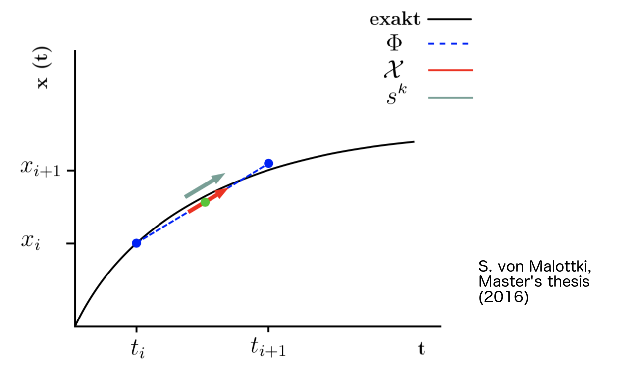
In the midpoint method the explicit and implicit Euler methods are combined.
With Φ = (f(x_i) + f(x_i+1))/2 this yields

x_i+1 = x_i + Δt_i (f(x_i+1) + f(x_i+1))/2

so a average slope is calculated and taken into account. A sketch can be seen in the following graph.

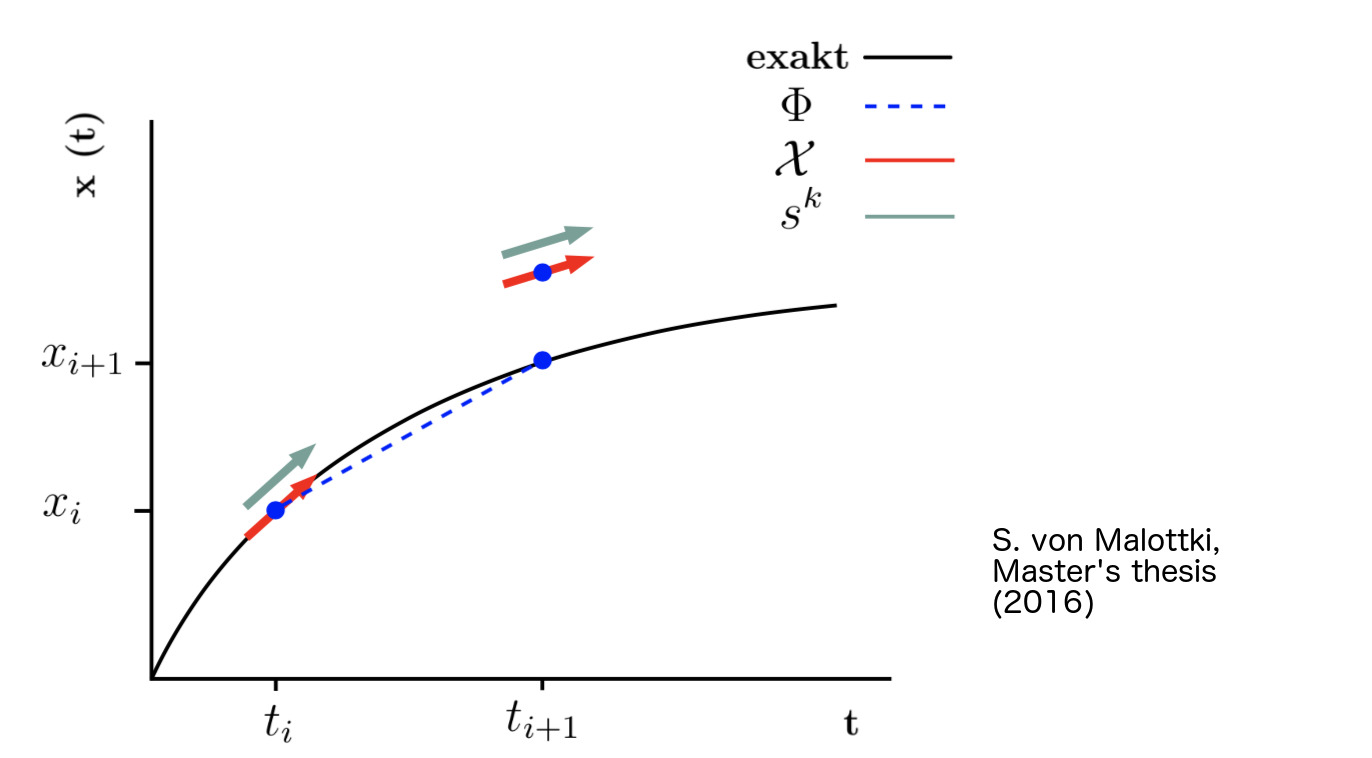
In this method is similar to the midpoint method, but x_i+1 is first calculated with the explicit Euler method (x_i+1 = x_i + Δt_i f(x_i)), so Φ = (f(x_i) + f(x_i + Δt_i f(x_i)))/2. With this, the Heun method is a explicit one step method with the calculation specification:

x_i+1 = x_i + Δt_i (f(x_i) + f(x_i + Δt_i f(x_i)))/2

A sketch can be seen in the following graph.

This method after Mentik et al. (2010) was proposed to solve the LL equation.

In the SIB method, two steps are made, a predicator step (first rough estimation of the integration) and a corrector step, which includes the predicator step.

In the predictor step, the midpoint method is applied, but the implicit calculation of the effective field is replaced by an explicit one

H_j,eff ((X_j+ X_j+1)/2) ->H_j,eff (X_j)

where different magnetic moments are now indicated by j.

In the corrector step, again the midpoint method is applied and but now, the effective field is calculated from the starting point and the predictor point.

H_j,eff ((X_j+ X_j+1)/2) ->H_j,eff ((X_j+ X_predictor)/2

A sketch of the predictor (left) and corrector (right) step is shown in the figure below.

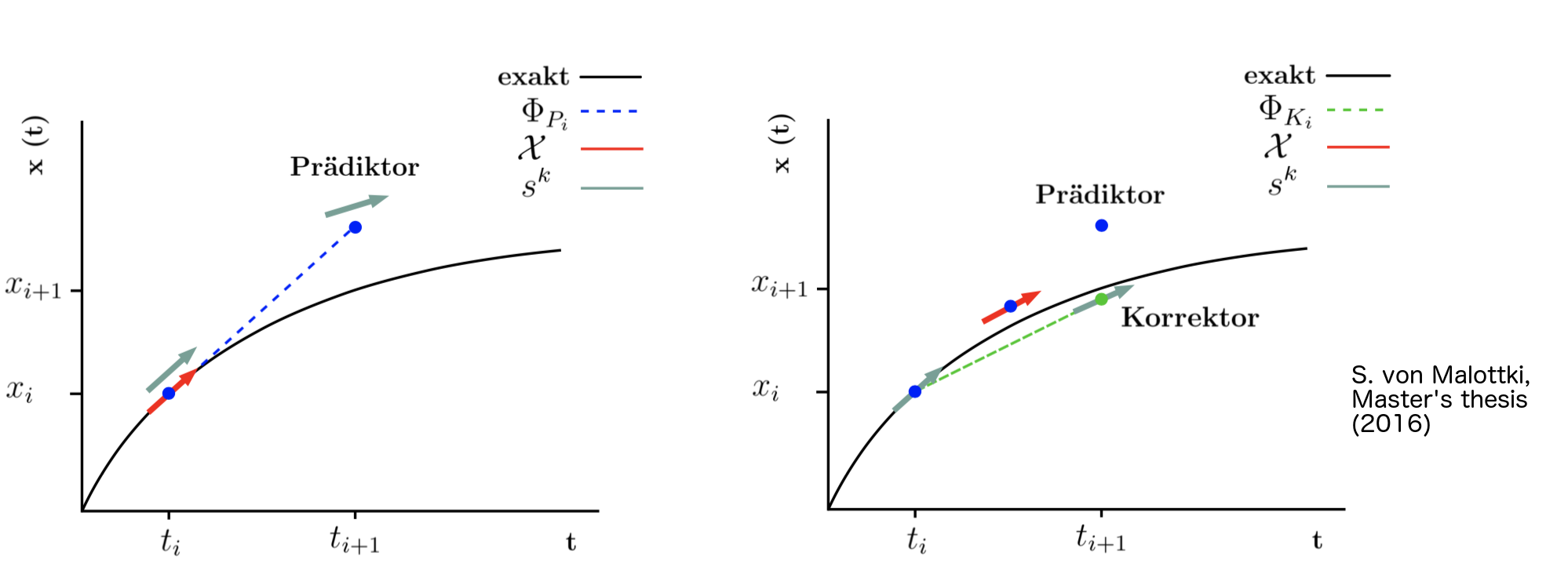
• C. Schieback, PhD thesis (2010)
• S. von Malottki, Master’s thesis (2016)
• Mentink et al., Journal of Physics: Condensed Matter 22, 17(2010)